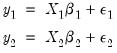
Denote a system of  equations in stacked form as:
equations in stacked form as: equations in stacked form as: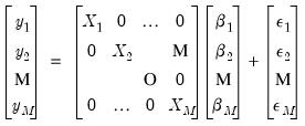 | (43.8) |
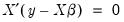
 is
is  vector,
  is a
is a  matrix, and
  is a
is a  vector of coefficients. The error terms
  have an
  covariance matrix
  . The system may be written in compact form as:
 | (43.9) |
 | (43.10) |
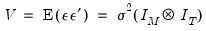
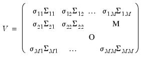
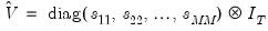
 equations. Second, they may be heteroskedastic and contemporaneously correlated. We can characterize both of these cases by defining the
  matrix of contemporaneous correlations,
  , where the (i,j)-th element of
  is given by
 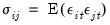 for all
  . If the errors are contemporaneously uncorrelated, then,
  for
for  , and we can write:
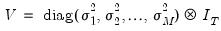 | (43.11) |
 | (43.12) |
 | (43.13) |
 is an autocorrelation matrix for the i-th and j-th equations.
 . The estimator for
  is given by,
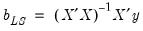 | (43.14) |
 | (43.15) |
 is the residual variance estimate for the stacked system.
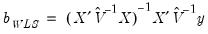 | (43.16) |
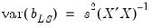
 is a consistent estimator of
  , and
, and  is the residual variance estimator:
 | (43.17) |
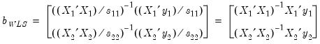
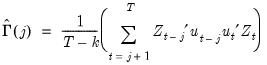
 and
and  . The max function in
Equation (43.17) is designed to handle the case of unbalanced data by down-weighting the covariance terms. Provided the missing values are asymptotically negligible, this yields a consistent estimator of the variance elements. Note also that there is no adjustment for degrees of freedom.
. The max function in
Equation (43.17) is designed to handle the case of unbalanced data by down-weighting the covariance terms. Provided the missing values are asymptotically negligible, this yields a consistent estimator of the variance elements. Note also that there is no adjustment for degrees of freedom. . If you choose not to iterate the weights, the OLS coefficient estimates will be used to estimate the variances. If you choose to iterate the weights, the current parameter estimates (which may be based on the previously computed weights) are used in computing the
  . This latter procedure may be iterated until the weights and coefficients converge.
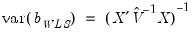 | (43.18) |
 | (43.19) |
 | (43.20) |
 are assumed to be exogenous, and the errors are heteroskedastic and contemporaneously correlated so that the error variance matrix is given by
  . Zellner’s SUR estimator of
  takes the form:
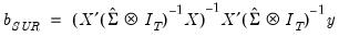 | (43.21) |
 is a consistent estimate of
  with typical element
  , for all
  and
and  .
. , EViews transforms the model (see
“Specifying AR Terms”) and estimates the following equation:
, EViews transforms the model (see
“Specifying AR Terms”) and estimates the following equation: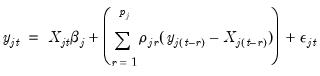 | (43.22) |
 is assumed to be serially independent, but possibly correlated contemporaneously across equations. At the beginning of the first iteration, we estimate the equation by nonlinear LS and use the estimates to compute the residuals
  . We then construct an estimate of
  using
using 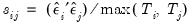 and perform nonlinear GLS to complete one iteration of the estimation procedure. These iterations may be repeated until the coefficients and weights converge.
 are endogenous. Write the j-th equation of the system as,
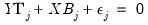 | (43.23) |
 | (43.24) |
 ,
,  ,
,  and
and  .
.  is the matrix of endogenous variables and
  is the matrix of exogenous variables;
  is the matrix of endogenous variables not including
  .
. on all exogenous variables
  and get the fitted values:
 | (43.25) |
 on
on  and
and  to get:
 | (43.26) |
 . The residuals from an equation using these coefficients are used for form weights.
 | (43.27) |
 is estimated at each step using the current values of the coefficients and residuals.
 . This covariance estimator is not, however, consistent if any of the right-hand side variables are endogenous. 3SLS uses the 2SLS residuals to obtain a consistent estimate of
  .
.  | (43.28) |
 has typical element:
 | (43.29) |
 .
. | (43.30) |
 is a vector of endogenous variables,
  is a vector of exogenous variables. The Full Information Maximum Likelihood (FIML) estimator finds the vector of parameters
  by maximizing the likelihood under the assumption that
  is a vector of i.i.d. multivariate normal random variables with covariance matrix
  .
. | (43.31) |
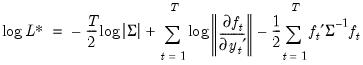
 . Note that the log determinant of the derivatives of
  captures the simultaneity in the system of equations.
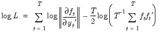 | (43.32) |
 (or equivalently, the full likelihood with respect to
  and the free parameters of
  ).
). given the user specified value for
  .
. is asymptotically normally distributed with coefficient covariance typically computed using the partitioned inverse of the outer-product of the gradient of the full likelihood (OPG) or the inverse of the negative of the observed Hessian of the concentrated likelihood. EViews employs the OPG covariance by default, but there is evidence that one should take seriously the choice of method (Calzolari and Panattoni, 1988). In addition, EViews offers a QML covariance computation that employs a Huber-White sandwich using both the OPG and the inverse negative Hessian.
 should satisfy. We denote these moment conditions as:
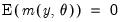 | (43.33) |
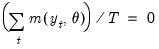 | (43.34) |
 when there are more restrictions
  than there are parameters
  . To allow for such overidentification, the GMM estimator is defined by minimizing the following criterion function:
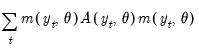 | (43.35) |
 and zero.
  is a weighting matrix that weights each moment condition. Any symmetric positive definite matrix
  will yield a consistent estimate of
  . However, it can be shown that a necessary (but not sufficient) condition to obtain an (asymptotically) efficient estimate of
  is to set
  equal to the inverse of the covariance matrix
  of the sample moments
  . This follows intuitively, since we want to put less weight on the conditions that are more imprecise.
  , and a set of instrumental variables,
  , so that:
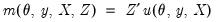 | (43.36) |
 | (43.37) |
 as there are parameters
  . See the section on
“Generalized Method of Moments” for additional examples of GMM orthogonality conditions.
. See the section on
“Generalized Method of Moments” for additional examples of GMM orthogonality conditions. . EViews uses the optimal
  , where
  is the estimated long-run covariance matrix of the sample moments
  . EViews uses the consistent TSLS estimates for the initial estimate of
  in forming the estimate of
  .
.  using White’s heteroskedasticity consistent covariance matrix:
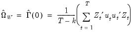 | (43.38) |
 is the vector of residuals, and
  is a
is a  matrix such that the
  moment conditions at
  may be written as
 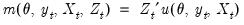 .
. by,
by,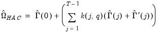 | (43.39) |
 | (43.40) |
 and the bandwidth
  .
.  is used to weight the covariances so that
  is ensured to be positive semi-definite. EViews provides two choices for the kernel, Bartlett and quadratic spectral (QS). The Bartlett kernel is given by:
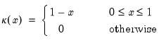 | (43.41) |
 | (43.42) |
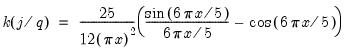
 . The QS has a faster rate of convergence than the Bartlett and is smooth and not truncated (Andrews 1991). Note that even though the QS kernel is not truncated, it still depends on the bandwidth
  (which need not be an integer).
  determines how the weights given by the kernel change with the lags in the estimation of
  . Newey-West fixed bandwidth is based solely on the number of observations in the sample and is given by:
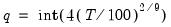 | (43.43) |
 | (43.44) |
 and
and  .
.  and the residual variances
  for
for  . Then
  and
and  are estimated by:
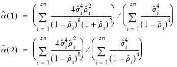 | (43.45) |
 .
.  and
and  are estimated by,
 | (43.46) |
 is a vector of ones and:
  | (43.47) |
 .
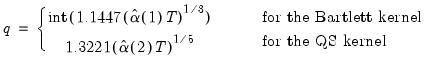
. . The choice of
  is arbitrary, subject to the condition that it grow at a certain rate. EViews sets the lag parameter to:
 | (43.48) |
 for the Bartlett kernel and
  for the quadratic spectral kernel.
 to “soak up” the correlations in
  prior to GMM estimation. We first fit a VAR(1) to the sample moments:
 | (43.49) |
 of
of  is estimated by
 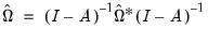 where
where  is the long-run variance of the residuals
  computed using any of the above methods. The GMM estimator is then found by minimizing the criterion function:
 | (43.50) |
 | (43.51) |
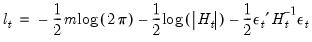
 is the
  vector of mean equation residuals. For Student's t-distribution, the contributions are of the form:
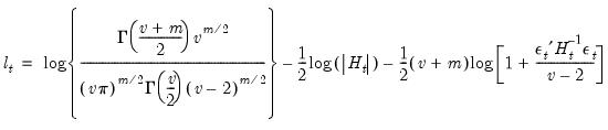 | (43.52) |
 is the estimated degree of freedom.
 | (43.53) |
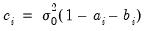
 ,
,  , and
, and  are
are  symmetric matrices, and the operator “•”is the element by element (Hadamard) product. The coefficient matrices may be parametrized in several ways. The most general way is to allow the parameters in the matrices to vary without any restrictions, i.e. parameterize them as indefinite matrices. In that case the model may be written in single equation format as:
 | (43.54) |
 is the i-th row and j-th column of matrix
  .
. parameters. This model is the most unrestricted version of a Diagonal VECH model. At the same time, it does not ensure that the conditional covariance matrix is positive semidefinite (PSD). As summarized in Ding and Engle (2001), there are several approaches for specifying coefficient matrices that restrict
  to be PSD, possibly by reducing the number of parameters. One example is:
 | (43.55) |
 ,
,  , and
, and  are any matrix up to rank
  . For example, one may use the rank
  Cholesky factorized matrix of the coefficient matrix. This method is labeled the Full Rank Matrix in the coefficient Restriction selection of the system ARCH dialog. While this method contains the same number of parameters as the indefinite version, it does ensure that the conditional covariance is PSD.
 and guarantees that the conditional covariance is PSD. In this case, the estimated raw matrix is restricted, with all but the first column of coefficients equal to zero.
 ,
,  , and
, and  . These coefficients must be transformed to obtain the matrix of interest:
  ,
,  , and
, and  . These transformed coefficients are reported in the extended variance coefficient section at the end of the system estimation results.
 matrix may be a constant, so that:
 | (43.56) |
 is a scalar and
  is an
is an  vector of ones. This Scalar specification implies that for a particular term, the parameters of the variance and covariance equations are restricted to be the same. Alternately, the matrix coefficients may be parameterized as Diagonal so that all off diagonal elements are restricted to be zero. In both of these parameterizations, the coefficients are not restricted to be positive, so that
  is not guaranteed to be PSD.
 , we may also impose a Variance Target on the coefficients which restricts the values of the coefficient matrix so that:
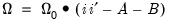 | (43.57) |
 is the unconditional sample variance of the residuals. When using this option, the constant matrix is not estimated, reducing the number of estimated parameters.
 , instead of
  .
. | (43.58) |
 | (43.59) |
 is the unconditional variance.
 , for every equation. Individual coefficients allow each exogenous variable effect
  to differ across equations.
 | (43.60) |
 | (43.61) |
 and
and  are unrestricted. However, a common and popular form, diagonal BEKK, may be specified that restricts
  and
and  to be diagonals. This Diagonal BEKK model is identical to the Diagonal VECH model where the coefficient matrices are rank one matrices. For convenience, EViews provides an option to estimate the Diagonal VECH model, but display the result in Diagonal BEKK form.
 and
and  are unrestricted, the WLS estimator given in