Coefficient Diagnostics
These diagnostics provide information and evaluate restrictions on the estimated coefficients, including the special case of tests for omitted and redundant variables.
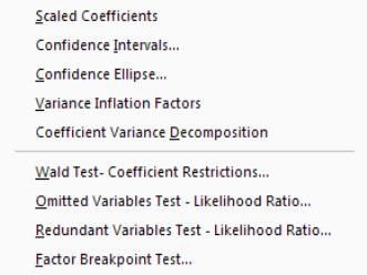
Scaled Coefficients
The view displays the coefficient estimates, the standardized coefficient estimates and the elasticity at means. The standardized coefficients are the point estimates of the coefficients standardized by multiplying by the standard deviation of the regressor divided by the standard deviation of the dependent variable.
The elasticity at means are the point estimates of the coefficients scaled by the mean of the dependent variable divided by the mean of the regressor.
Confidence Intervals and Confidence Ellipses
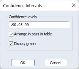
The view displays a table of confidence intervals for each of the coefficients in the equation.
The dialog allows you to enter the size of the confidence levels. These can be entered a space delimited list of decimals, or as the name of a scalar or vector in the workfile containing confidence levels. You can also choose how you would like to display the confidence intervals. By default they will be shown in pairs where the low and high values for each confidence level are shown next to each other. By unchecking the checkbox you can choose to display the confidence intervals concentrically.
The view plots the joint confidence region of any two functions of estimated parameters from an EViews estimation object. Along with the ellipses, you can choose to display the individual confidence intervals.
We motivate our discussion of this view by pointing out that the Wald test view () allows you to test restrictions on the estimated coefficients from an estimation object. When you perform a Wald test, EViews provides a table of output showing the numeric values associated with the test.
An alternative approach to displaying the results of a Wald test is to display a confidence interval. For a given test size, say 5%, we may display the one-dimensional interval within which the test statistic must lie for us not to reject the null hypothesis. Comparing the realization of the test statistic to the interval corresponds to performing the Wald test.
The one-dimensional confidence interval may be generalized to the case involving two restrictions, where we form a joint confidence region, or confidence ellipse. The confidence ellipse may be interpreted as the region in which the realization of two test statistics must lie for us not to reject the null.
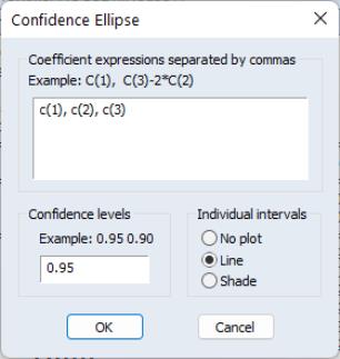
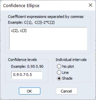
To display confidence ellipses in EViews, simply select from the estimation object toolbar. EViews will display a dialog prompting you to specify the coefficient restrictions and test size, and to select display options.
The first part of the dialog is identical to that found in the Wald test view—here, you will enter your coefficient restrictions into the edit box, with multiple restrictions separated by commas. The computation of the confidence ellipse requires a minimum of two restrictions. If you provide more than two restrictions, EViews will display all unique pairs of confidence ellipses.
In this simple example depicted here using equation EQ01 from the workfile “Cellipse.WF1”, we provide a (comma separated) list of coefficients from the estimated equation. This description of the restrictions takes advantage of the fact that EViews interprets any expression without an explicit equal sign as being equal to zero (so that “C(1)” and “C(1)=0” are equivalent). You may, of course, enter an explicit restriction involving an equal sign (for example, “C(1)+C(2) = C(3)/2”).
Next, select a size or sizes for the confidence ellipses. Here, we instruct EViews to construct a 95% confidence ellipse. Under the null hypothesis, the test statistic values will fall outside of the corresponding confidence ellipse 5% of the time.
Lastly, we choose a display option for the individual confidence intervals. If you select or , EViews will mark the confidence interval for each restriction, allowing you to see, at a glance, the individual results. will display the individual confidence intervals as dotted lines; will display the confidence intervals as a shaded region. If you select , EViews will not display the individual intervals.
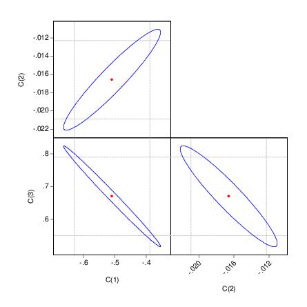
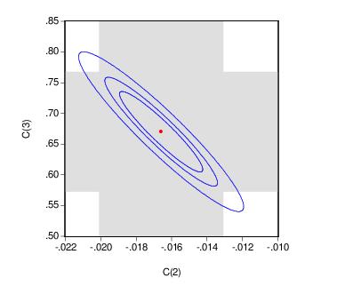
The output depicts three confidence ellipses that result from pairwise tests implied by the three restrictions (“C(1)=0”, “C(2)=0”, and “C(3)=0”).
Notice first the presence of the dotted lines showing the corresponding confidence intervals for the individual coefficients.
The next thing that jumps out from this example is that the coefficient estimates are highly correlated—if the estimates were independent, the ellipses would be exact circles.
You can easily see the importance of this correlation. For example, focusing on the ellipse for C(1) and C(3) depicted in the lower left-hand corner, an estimated C(1) of –.65 is sufficient reject the hypothesis that C(1)=0 (since it falls below the end of the univariate confidence interval). If C(3)=.8, we cannot reject the joint null that C(1)=0, and C(3)=0 (since C(1)=-.65, C(3)=.8 falls within the confidence ellipse).
EViews allows you to display more than one size for your confidence ellipses. This feature allows you to draw confidence contours so that you may see how the rejection region changes at different probability values. To do so, simply enter a space delimited list of confidence levels. Note that while the coefficient restriction expressions must be separated by commas, the contour levels must be separated by spaces.
Here, the individual confidence intervals are depicted with shading. The individual intervals are based on the largest size confidence level (which has the widest interval), in this case, 0.9.
Computational Details
Consider two functions of the parameters

and

, and define the bivariate function
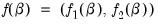
.
The size

joint confidence ellipse is defined as the set of points

such that:
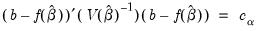 | (26.1) |
where

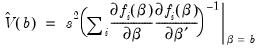
are the parameter estimates,

is the covariance matrix of

, and

is the size

critical value for the related distribution. If the parameter estimates are least-squares based, the

distribution is used; if the parameter estimates are likelihood based, the

distribution will be employed.
The individual intervals are two-sided intervals based on either the
t-distribution (in the cases where

is computed using the
F-distribution), or the normal distribution (where

is taken from the

distribution).
Variance Inflation Factors
(VIFs) are a method of measuring the level of collinearity between the regressors in an equation. VIFs show how much of the variance of a coefficient estimate of a regressor has been inflated due to collinearity with the other regressors. They can be calculated by simply dividing the variance of a coefficient estimate by the variance of that coefficient had other regressors not been included in the equation.
There are two forms of the Variance Inflation Factor: centered and uncentered. The centered VIF is the ratio of the variance of the coefficient estimate from the original equation divided by the variance from a coefficient estimate from an equation with only that regressor and a constant. The uncentered VIF is the ratio of the variance of the coefficient estimate from the original equation divided by the variance from a coefficient estimate from an equation with only one regressor (and no constant). Note that if you original equation did not have a constant only the uncentered VIF will be displayed.
The VIF view for EQ01 from the “Cellipse.WF1” workfile contains:
The centered VIF is numerically identical to

where

is the R-squared from the regression of that regressor on all of the other regressors in the equation.
Note that since the VIFs are calculated from the coefficient variance-covariance matrix, any robust standard error options will be present in the VIFs.
Coefficient Variance Decomposition
The Coefficient Variance Decomposition view of an equation provides information on the eigenvector decomposition of the coefficient covariance matrix. This decomposition is a useful tool to help diagnose potential collinearity problems amongst the regressors. The decomposition calculations follow those given in Belsley, Kuh and Welsch (BKW) 2004 (Section 3.2). Note that although BKW use the singular-value decomposition as their method to decompose the variance-covariance matrix, since this matrix is a square positive semi-definite matrix, using the eigenvalue decomposition will yield the same results.
In the case of a simple linear least squares regression, the coefficient variance-covariance matrix can be decomposed as follows:
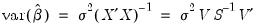 | (26.2) |
where

is a diagonal matrix containing the eigenvalues of

, and

is a matrix whose columns are equal to the corresponding eigenvectors.
The variance of an individual coefficient estimate is then:
 | (26.3) |
where

is the
j-th eigenvalue, and

is the (
i,
j)-th element of

.
We term the
j-th condition number of the covariance matrix,

:
 | (26.4) |
If we let:
 | (26.5) |
and
 | (26.6) |
then we can term the variance-decomposition proportion as:
 | (26.7) |
These proportions, together with the condition numbers, can then be used as a diagnostic tool for determining collinearity between each of the coefficients.
Belsley, Kuh and Welsch recommend the following procedure:
• Check the condition numbers of the matrix. A condition number smaller than 1/900 (0.001) could signify the presence of collinearity. Note that BKW use a rule of any number greater than 30, but base it on the condition numbers of

, rather than

.
• If there are one or more small condition numbers, then the variance-decomposition proportions should be investigated. Two or more variables with values greater than 0.5 associated with a small condition number indicate the possibility of collinearity between those two variables.
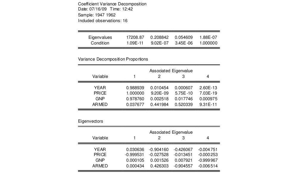
To view the coefficient variance decomposition in EViews, select . EViews will then display a table showing the Eigenvalues, Condition Numbers, corresponding Variance Decomposition Proportions and, for comparison purposes, the corresponding Eigenvectors.
As an example, we estimate an equation using data from Longley (1967), as republished in Greene (2008). The workfile “Longley.WF1” contains macro economic variables for the US between 1947 and 1962, and is often used as an example of multicollinearity in a data set. The equation we estimate regresses Employment on Year (YEAR), the GNP Deflator (PRICE), GNP, and Armed Forces Size (ARMED). The coefficient variance decomposition for this equation is show below.
The top line of the table shows the eigenvalues, sorted from largest to smallest, with the condition numbers below. Note that the final condition number is always equal to 1. Three of the four eigenvalues have condition numbers smaller than 0.001, with the smallest condition number being very small: 1.09E-11, which would indicate a large amount of collinearity.
The second section of the table displays the decomposition proportions. The proportions associated with the smallest condition number are located in the first column. Three of these values are larger than 0.5, indeed they are very close to 1. This indicates that there is a high level of collinearity between those three variables, YEAR, PRICE and GNP.
Wald Test (Coefficient Restrictions)
The Wald test computes a test statistic based on the unrestricted regression. The Wald statistic measures how close the unrestricted estimates come to satisfying the restrictions under the null hypothesis. If the restrictions are in fact true, then the unrestricted estimates should come close to satisfying the restrictions.
How to Perform Wald Coefficient Tests
To demonstrate the calculation of Wald tests in EViews, we consider simple examples. Suppose a Cobb-Douglas production function has been estimated in the form:
 | (26.8) |
where

,

and

denote value-added output and the inputs of capital and labor respectively. The hypothesis of constant returns to scale is then tested by the restriction:

.
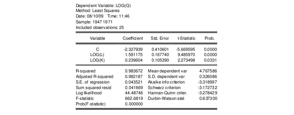
Estimation of the Cobb-Douglas production function using annual data from 1947 to 1971 in the workfile “Coef_test.WF1” provided the following result:
The sum of the coefficients on LOG(L) and LOG(K) appears to be in excess of one, but to determine whether the difference is statistically relevant, we will conduct the hypothesis test of constant returns.
To carry out a Wald test, choose from the equation toolbar. Enter the restrictions into the edit box, with multiple coefficient restrictions separated by commas. The restrictions should be expressed as equations involving the estimated coefficients and constants. The coefficients should be referred to as C(1), C(2), and so on, unless you have used a different coefficient vector in estimation.
If you enter a restriction that involves a series name, EViews will prompt you to enter an observation at which the test statistic will be evaluated. The value of the series will at that period will be treated as a constant for purposes of constructing the test statistic.
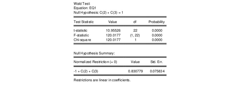
To test the hypothesis of constant returns to scale, type the following restriction in the dialog box:
c(2) + c(3) = 1
and click OK. EViews reports the following result of the Wald test:
EViews reports an
F-statistic and a Chi-square statistic with associated
p-values. In cases with a single restriction, EViews reports the
t-statistic equivalent of the
F-statistic. See
“Wald Test Details” for a discussion of these statistics. In addition, EViews reports the value of the normalized (homogeneous) restriction and an associated standard error. In this example, we have a single linear restriction so the
F-statistic and Chi-square statistic are identical, with the
p-value indicating that we can decisively reject the null hypothesis of constant returns to scale.
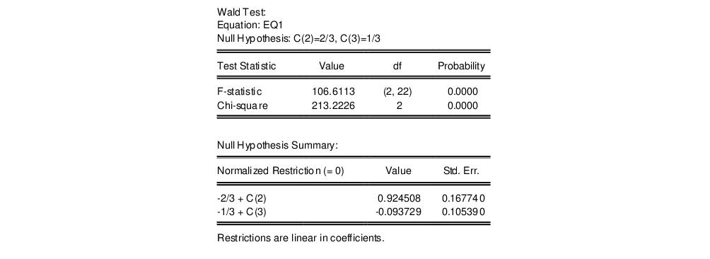
To test more than one restriction, separate the restrictions by commas. For example, to test the hypothesis that the elasticity of output with respect to labor is 2/3 and the elasticity with respect to capital is 1/3, enter the restrictions as,
c(2)=2/3, c(3)=1/3
and EViews reports:
Note that in addition to the test statistic summary, we report the values of both of the normalized restrictions, along with their standard errors (the square roots of the diagonal elements of the restriction covariance matrix).
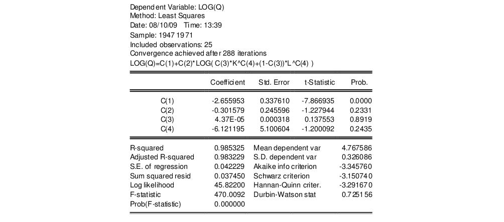
As an example of a nonlinear model with a nonlinear restriction, we estimate a general production function of the form:
 | (26.9) |
and test the constant elasticity of substitution (CES) production function restriction

. This is an example of a nonlinear restriction. To estimate the (unrestricted) nonlinear model, you may initialize the parameters using the command
param c(1) -2.6 c(2) 1.8 c(3) 1e-4 c(4) -6
then select and then estimate the following specification:
log(q) = c(1) + c(2)*log(c(3)*k^c(4)+(1-c(3))*l^c(4))
to obtain
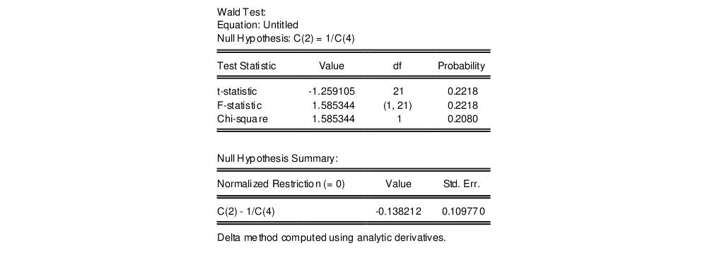
To test the nonlinear restriction

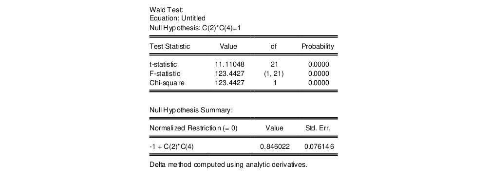
, choose from the equation toolbar and type the following restriction in the Wald Test dialog box:
c(2)=1/c(4)
The results are presented below:
We focus on the p-values for the statistics which show that we fail to reject the null hypothesis. Note that EViews reports that it used the delta method (with analytic derivatives) to compute the Wald restriction variance for the nonlinear restriction.
It is well-known that nonlinear Wald tests are not invariant to the way that you specify the nonlinear restrictions. In this example, the nonlinear restriction

may equivalently be written as

or

(for nonzero

and

). For example, entering the restriction as,
c(2)*c(4)=1
yields:
so that the test now decisively rejects the null hypothesis. We hasten to add that this type of inconsistency in results is not unique to EViews, but is a more general property of the Wald test. Unfortunately, there does not seem to be a general solution to this problem (see Davidson and MacKinnon, 1993, Chapter 13).
Wald Test Details
Consider a general nonlinear regression model:
 | (26.10) |
where

and

are

-vectors and

is a

-vector of parameters to be estimated. Any restrictions on the parameters can be written as:
 | (26.11) |
where

is a smooth function,

, imposing

restrictions on

. The Wald statistic is then computed as:
 | (26.12) |
where

is the number of observations and

is the vector of unrestricted parameter estimates, and where

is an estimate of the

covariance. In the standard regression case,

is given by:
 | (26.13) |
where

is the vector of unrestricted residuals, and

is the usual estimator of the unrestricted residual variance,
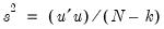
, but the estimator of

may differ. For example,

may be a robust variance matrix estimator computing using White or Newey-West techniques.
More formally, under the null hypothesis

, the Wald statistic has an asymptotic

distribution, where

is the number of restrictions under

.
For the textbook case of a linear regression model,
 | (26.14) |
and linear restrictions:
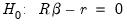 | (26.15) |
where

is a known

matrix, and

is a

-vector, respectively. The Wald statistic in
Equation (26.12) reduces to:
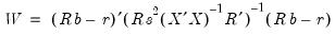 | (26.16) |
which is asymptotically distributed as

under

.
If we further assume that the errors

are independent and identically normally distributed, we have an exact, finite sample
F-statistic:
 | (26.17) |
where

is the vector of residuals from the restricted regression. In this case, the
F-statistic compares the residual sum of squares computed with and without the restrictions imposed.
We remind you that the expression for the finite sample
F-statistic in
(26.17) is for standard linear regression, and is not valid for more general cases (nonlinear models, ARMA specifications, or equations where the variances are estimated using other methods such as Newey-West or White). In non-standard settings, the reported
F-statistic (which EViews always computes as

), does not possess the desired finite-sample properties. In these cases, while asymptotically valid,
F-statistic (and corresponding
t-statistic) results should be viewed as illustrative and for comparison purposes only.
Omitted Variables
This test enables you to add a set of variables to an existing equation and to ask whether the set makes a significant contribution to explaining the variation in the dependent variable. The null hypothesis

is that the additional set of regressors are not jointly significant.
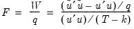
The output from the test is an F-statistic and a likelihood ratio (LR) statistic with associated p-values, together with the estimation results of the unrestricted model under the alternative. The F-statistic is based on the difference between the residual sums of squares of the restricted and unrestricted regressions and is only valid in linear regression based settings. The LR statistic is computed as:
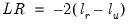 | (26.18) |
where

and

are the maximized values of the (Gaussian) log likelihood function of the unrestricted and restricted regressions, respectively. Under

, the LR statistic has an asymptotic

distribution with degrees of freedom equal to the number of restrictions (the number of added variables).
Bear in mind that:
• The omitted variables test requires that the same number of observations exist in the original and test equations. If any of the series to be added contain missing observations over the sample of the original equation (which will often be the case when you add lagged variables), the test statistics cannot be constructed.
• The omitted variables test can be applied to equations estimated with linear LS, ARCH (mean equation only), binary, ordered, censored, truncated, and count models. The test is available only if you specify the equation by listing the regressors, not by a formula.
• Equations estimated by Two-Stage Least Squares and GMM offer a variant of this test based on the difference in J-statistics.
To perform an LR test in these settings, you can estimate a separate equation for the unrestricted and restricted models over a common sample, and evaluate the LR statistic and p-value using scalars and the @cchisq function, as described above.
How to Perform an Omitted Variables Test
To test for omitted variables, select In the dialog that opens, list the names of the test variables, each separated by at least one space. Suppose, for example, that the initial regression specification is:
log(q) c log(l) log(k)
If you enter the list:
log(l)^2 log(k)^2
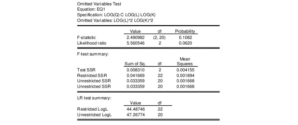
in the dialog, then EViews reports the results of the unrestricted regression containing the two additional explanatory variables, and displays statistics testing the hypothesis that the coefficients on the new variables are jointly zero. The top part of the output depicts the test results (the bottom portion shows the estimated test equation):
The
F-statistic has an exact finite sample
F-distribution under

for linear models if the errors are independent and identically distributed normal random variables. The numerator degrees of freedom is the number of additional regressors and the denominator degrees of freedom is the number of observations less the total number of regressors. The log likelihood ratio statistic is the LR test statistic and is asymptotically distributed as a

with degrees of freedom equal to the number of added regressors.
In our example, neither test rejects the null hypothesis that the two series do not belong to the equation at a 5% significance level.
Redundant Variables
The redundant variables test allows you to test for the statistical significance of a subset of your included variables. More formally, the test is for whether a subset of variables in an equation all have zero coefficients and might thus be deleted from the equation. The redundant variables test can be applied to equations estimated by linear LS, TSLS, ARCH (mean equation only), binary, ordered, censored, truncated, and count methods. The test is available only if you specify the equation by listing the regressors, not by a formula.
How to Perform a Redundant Variables Test
To test for redundant variables, select In the dialog that appears, list the names of each of the test variables, separated by at least one space. Suppose, for example, that the initial regression specification is:
log(q) c log(l) log(k) log(l)^2 log(k)^2
If you type the list:
log(l)^2 log(k)^2
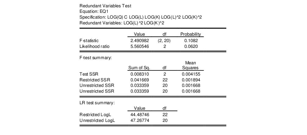
in the dialog, then EViews reports the results of the restricted regression dropping the two regressors, followed by the statistics associated with the test of the hypothesis that the coefficients on the two variables are jointly zero. The top portion of the output is:
The reported test statistics are the
F-statistic and the Log likelihood ratio. The
F-statistic has an exact finite sample
F-distribution under

if the errors are independent and identically distributed normal random variables and the model is linear. The numerator degrees of freedom are given by the number of coefficient restrictions in the null hypothesis. The denominator degrees of freedom are given by the total regression degrees of freedom. The LR test is an asymptotic test, distributed as a

with degrees of freedom equal to the number of excluded variables under

. In this case, there are two degrees of freedom.
Factor Breakpoint Test
The Factor Breakpoint test splits an estimated equation's sample into a number of subsamples classified by one or more variables and examines whether there are significant differences in equations estimated in each of those subsamples. A significant difference indicates a structural change in the relationship. For example, you can use this test to examine whether the demand function for energy differs between the different states of the USA. The test may be used with least squares and two-stage least squares regressions.
By default the Factor Breakpoint test tests whether there is a structural change in all of the equation parameters. However if the equation is linear EViews allows you to test whether there has been a structural change in a subset of the parameters.
To carry out the test, we partition the data by splitting the estimation sample into subsamples of each unique value of the classification variable. Each subsample must contain more observations than the number of coefficients in the equation so that the equation can be estimated. The Factor Breakpoint test compares the sum of squared residuals obtained by fitting a single equation to the entire sample with the sum of squared residuals obtained when separate equations are fit to each subsample of the data.
EViews reports three test statistics for the Factor Breakpoint test. The F-statistic is based on the comparison of the restricted and unrestricted sum of squared residuals and in the simplest case involving two subsamples, is computed as:
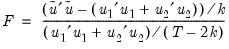 | (26.19) |
where

is the restricted sum of squared residuals,

is the sum of squared residuals from subsample

,

is the total number of observations, and

is the number of parameters in the equation. This formula can be generalized naturally to more than two subsamples. The
F-statistic has an exact finite sample
F-distribution if the errors are independent and identically distributed normal random variables.
The log likelihood ratio statistic is based on the comparison of the restricted and unrestricted maximum of the (Gaussian) log likelihood function. The LR test statistic has an asymptotic

distribution with degrees of freedom equal to

under the null hypothesis of no structural change, where

is the number of subsamples.
The Wald statistic is computed from a standard Wald test of the restriction that the coefficients on the equation parameters are the same in all subsamples. As with the log likelihood ratio statistic, the Wald statistic has an asymptotic

distribution with

degrees of freedom, where

is the number of subsamples.
For example, suppose we have estimated an equation specification of
lwage c grade age high
using data from the “Cps88.WF1” workfile.
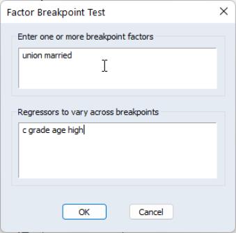
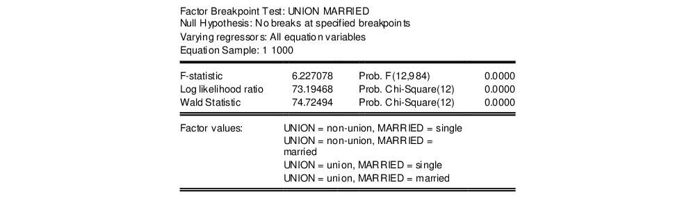
From this equation we can investigate whether the coefficient estimates on the wage equation differ by union membership and marriage status by using the UNION and MARRIED variables in a factor breakpoint test. To apply the breakpoint test, push on the equation toolbar. In the dialog that appears, list the series that will be used to classify the equation into subsamples. Since UNION contains values representing either union or non-union and MARRIED contains values for married and single, entering “union married” will specify 4 subsamples: non-union/married, non-union/single, union/married, and union/single. In the bottom portion of the dialog we indicate the names of the regressors that should be allowed to vary across breakpoints. By default, all of the variables will be allowed to vary.
This test yields the following result:
Note all three statistics decisively reject the null hypothesis.