Outlier Detection
The new equation outlier detection view offers two approaches to identifying outliers in an estimated equation.
• One set of equation outlier detection methods employs the series outlier methods
“Outlier Detection” applied to the residuals of the equation.
• The second set of methods computes influence statistic measures in equations estimated by least squares (Rstudent, HatMatrix, DFFITS, COVRATIO, and DFBETAS,
“Influence Statistics”) and uses them to identify outliers.
Performing Residual Outlier Diagnostics in EViews
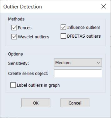
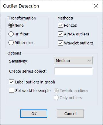
To perform outlier detection using the residuals from an equation in EViews, open the equation, and click on View/Outlier Diagnostics…. EViews will display the dialog:
The section offers checkboxes which select which of the outlier detection methods to use. The available options will depend on the method used to estimate the original equation.
• The and are only available for equations estimated by linear least squares.
• are only available for linear equations with ARMA terms.
Note that selecting the box will instruct EViews to employ both Tukey and Mean/Standard Deviation fences. Selecting will use Rstudent, HatMatrix, DFFITS, and COVRATIO.
The Options section has a number of options for tailoring the detection routine and its output.
• The Sensitivity drop down box allows you to quickly set the tolerance levels of the outlier detection methods. Sensitivity can be set to Low, Medium, High, or Custom. The values corresponding to the settings are:
| | | |
| 3.0 | 1.5 | 0.4 |
| 4.7 | 2.7 | 1.5 |
| 16.0 | 8.0 | 4.0 |
| 0.0005 | 0.001 | 0.01 |
| 4.0 | 3.0 | 2.0 |
| | | |
| | | |
| | | |
| | | |
where

is the number of regressors in the original equation, and

is the number of observations.
Note that the corresponds to

for the Tukey and Mean/Standard Deviation fences, the critical value

for several of the statistics, and the False Detection Rate (FDR) for wavelet analysis. Chen and Liu (1993, Section 3.1, p. 288) offer a simulation study which provides some guidance for the specification of the critical value

. If
Custom is selected, a new dialog will open, allowing setting of these values on an individual basis.
• If you enter a valid object name in the Create series object edit field EViews will produce a new binary series object in the workfile containing a value of “1” for any observation that was identified as an outlier, and a value of “0” for any observation that was not determined to be an outlier. Any observations outside of the current workfile sample are assigned a value of NA.
• Checking the Label outliers in graphs checkbox instructs EViews to include the date label of any identified outlier on the output graph.
An Example
We illustrate using an estimated equation taken from Wooldridge (2000, Example 9.8) for the regression of R&D expenditures (RDINTENS) on sales (SALES), profits (PROFITMARG), and a constant. The equation E1 in the workfile “RDChem.wf1” was used previously to illustrate the influence statistics view (
“Influence Statistics”).
Open the estimated equation E1, select to display the dialog:
and click on to accept the default settings. EViews displays a spool containing the results:
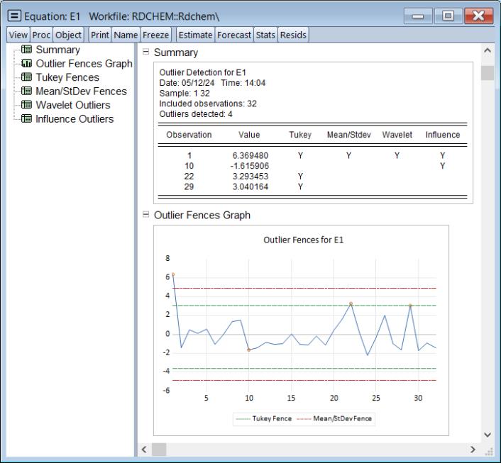
The shows that are four identified outliers. Observation 1 is an outlier in all four cases, while the remaining three observations are outliers under only one case.
The shows a plot of the equation residuals, with the four outliers identified, along with lines for both the Tukey and the Mean/StdDev fences.
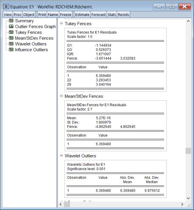
The , , and the results show computational details for each of the methods:
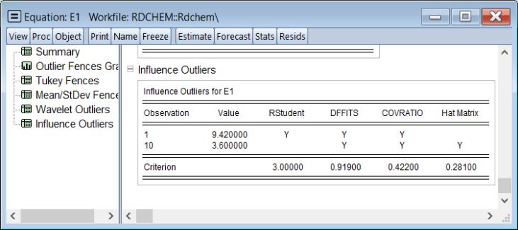
The table, which is only available for outlier determination from equation estimates, shows results for the individual criteria:
Note that both observations are deemed to be outliers by 3 of 4 evaluation methods.


 is the number of regressors in the original equation, and
  is the number of observations.
 for the Tukey and Mean/Standard Deviation fences, the critical value
  for several of the statistics, and the False Detection Rate (FDR) for wavelet analysis. Chen and Liu (1993, Section 3.1, p. 288) offer a simulation study which provides some guidance for the specification of the critical value
  . If Custom is selected, a new dialog will open, allowing setting of these values on an individual basis.