Examples
Below, we demonstrate VEC estimation using the EViews example workfile “var1.WF1”, located under the
“Vector Error Correction Models (VECMs)” folder. This is a workfile with a number of classic macroeconomic variables including gross domestic product, various measure of money supply, treasury bills of different maturations, industrial production, producer price index, the unemployment.
Example 1: Unrestricted Constant (JHJ)
We begin with the classical problem of studying the relationship between money supply (M1), gross domestic product (GDP), and 3-month Treasury bills (TB3).
These three endogenous variables will enter the VEC system with lags 1 through 4, and we assume that there exists a single cointegrating relationship. Furthermore, we will estimate the VEC using the default deterministic specification – . In this case, the constant is not restricted to the cointegrating relations, but is artificially inserted into the cointegrating vector using orthogonalization (
“The Johansen, Hendry, and Juselius Approach”).
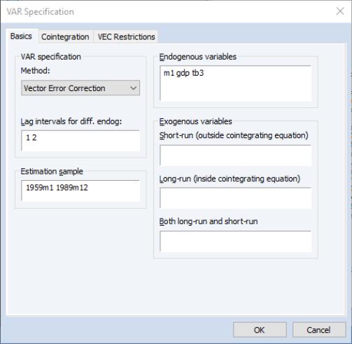
To estimate this model, select in the dropdown menu to display the VEC estimation dialog then enter “
m1 gdp tb3
in the field on the tab.
Furthermore, specify
1 4
in the field
and
1959m01 1982m03
in the edit field. We emphasize again that the lag interval specification refers to the differences of the dependent variable in the conditional error correction equation, and not the dependent variable itself in the levels equation.
You may leave the remaining fields and options at their default values. Hit to estimate the VEC with this specification. EViews will estimate the VEC and display the output in a table which contains four sections. Click on the button and enter .
At the top of the output, EViews shows a summary of the estimation procedure, including the sample, lag specification, variables, and deterministic assumptions used on constructing the estimates:
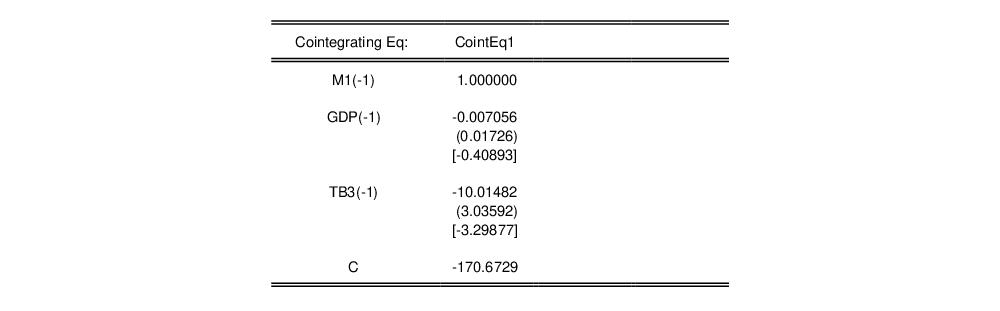
Next is a table of coefficient estimates for the cointegrating relation. In this case which is estimated assuming the default of one cointegrating vector, there is a single column of coefficients representing the only column of the cointegrating matrix. Since the deterministics are assumed to follow Johansen-Hendry-Juselius variant Case 3, the cointegrating relation includes an orthogonalized intercept estimate of -170.6729
Notably, there is no standard estimate for the orthogonalized intercept estimate.
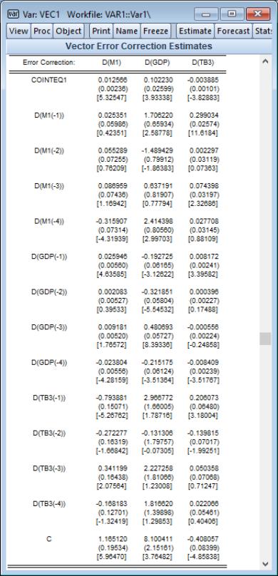
Next, EViews displays a table containing the coefficient estimates for the error correction regressions, with the results for each dependent variable appearing in columns.
The long-run portion of these results, the adjustment coefficients

, appear at the top of the table, as the estimated coefficient on COINTEQ1.
The remaining coefficients are estimates of the short-run-dynamics coefficients

. Note that for JHJ Case 3, the short-run results include estimates of the intercept, C. Since C is both inside and outside the cointegrating equation, keep in mind that the short-run estimate is obtained conditionally on the orthogonalized estimate of C in the cointegrating equation.
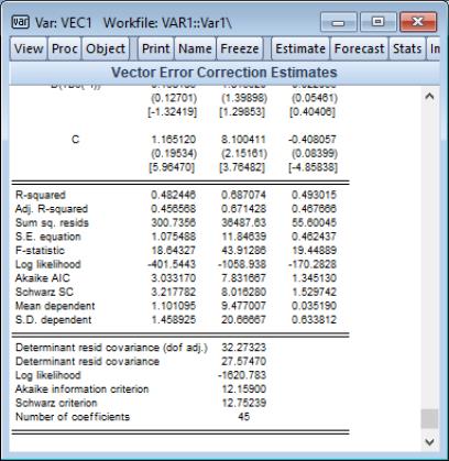
Just below the remainder of the short-run estimates including the estimate for C is the last part of the output showing summary statistics associated with the overall fit.
Example 2: Unrestricted Constant, Restricted Trend
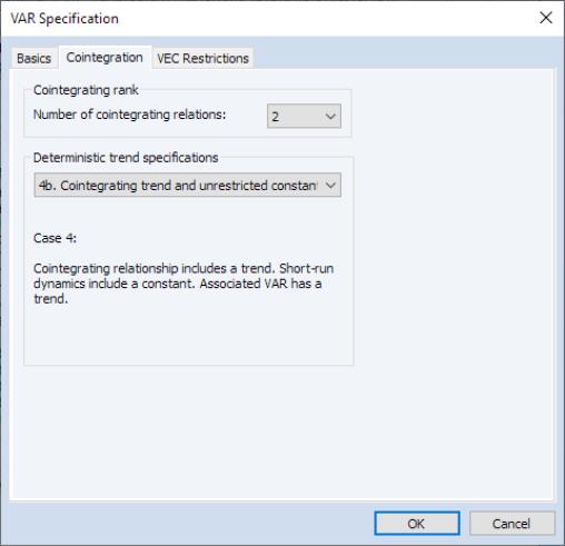
We modify the previous example to use only the first 2 lags, to have cointegration rank 2, and assume that the constant is entirely unrestricted, but restricting the trend to the cointegrating relation and the intercept to the short-run equation. To proceed, copy the existing var object, click on the button to bring up the VAR estimation dialog again, and then change the to “1 2”:
then click on the tab. select as the , and change the dropdown to .
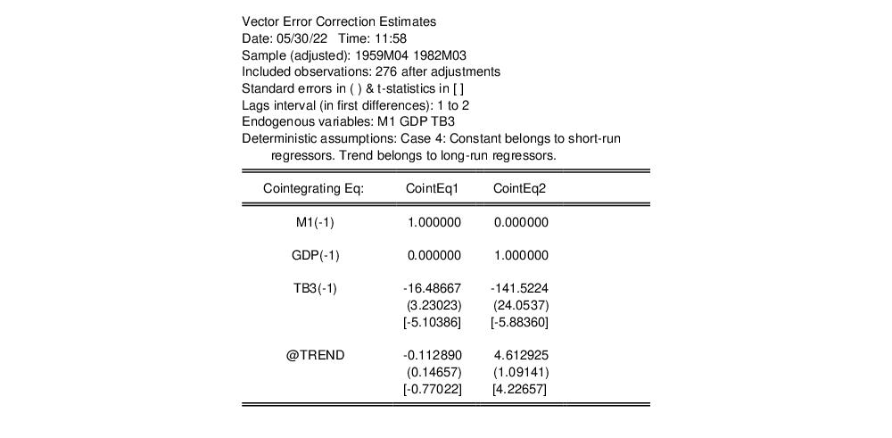
Click on to estimate the revised model, then press and enter VEC2. the top portion of the output is given by:
Notice that there are now two cointegrating vectors, and , which include a trend, with coefficient estimates -0.1129 and 4.6129, respectively, and standard errors, but not a constant since the latter is in the short-run regressors.
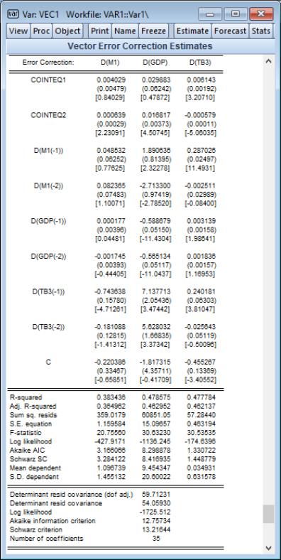
The error correction results, which now include the two cointegrated series COINTEQ1 and COINTEQ2, and an intercept, and the summary statistics results are presented below:
Example 3: Unrestricted Constant, Restricted Trend, and Exogenous
Extending the previous model, let us augment the cointegrating relation and the short-run dynamics by including exogenous variables. These exogenous variables can enter the cointegrating relation, so that they affect the long-run relationship, and they can be in the short-run relationship where they affect the dynamics of convergence to equilibrium.
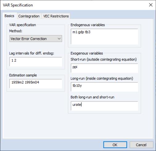
Let us assume that the 10-year Treasury bill rate (TB10Y) is an exogenous variable inside the cointegrating relation but not a part of the short-run dynamics, that the Producer Price Index (PPI), a measure of inflation, impacts only the short-run dynamics to convergence, and that the unemployment rate (UNRATE) is in both the short and long-run relationships.
Copy the existing var then click on to modify the specification. We enter “PPI” in the field, “TB10Y” in the field, and “URATE” in the field:
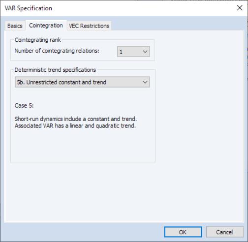
Furthermore, we’ll assume there’s a single cointegrating relation, and that the deterministic case specifies a constant and trend only affect the adjustment to equilibrium dynamics (short-run).
Click on the tab and change the dropdown to 1, and set the dropdown to :
Click on to estimate the updated specification.
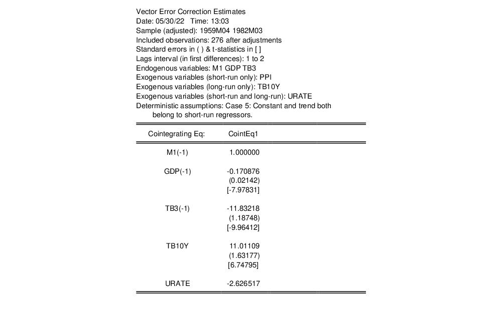
Notice that in addition to a description of the deterministic trend assumption, the output header now lists the exogenous variables included in the specification, by type.
Below the header, the results for the cointegrating vector show the three endogenous variables, followed by the coefficient for the long-run only variable TB10Y, and the both long and short-run variable URATE. Since the latter is included in the cointegrating equation via orthogonalization, is no standard error associated with the estimated coefficient.
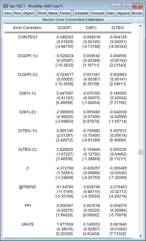
The error correction results include estimates for the two short-run only deterministic trend variables, C and @TREND, along with the short-run only PPI, and the both long and short-run URATE. As with other both long and short-run variables, the coefficient of URATE is estimated conditionally on the orthogonalization.
Example 4: VEC Restrictions
We may continue with the previous example after imposing restrictions on elements of the

matrix.
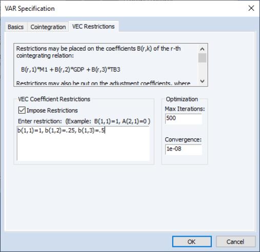
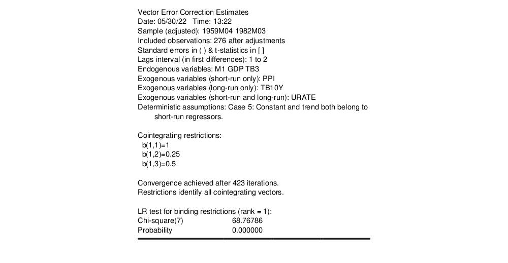
Once again, copy the existing var object, click on the button to bring up the VAR estimation dialog. Leave the existing specification in place, including the exogenous variables, but click on the tab to display the restrictions settings dialog. Click on the to enable the restrictions and enter “B(1,1)=1, B(1,2)=0.25, B(1,3)=0.5” in the edit field:
This specification restricts the first three elements of the cointegrating vector to the specified values. Click on to estimate the restricted VEC.
The familiar heading information is augmented to show the cointegrating restrictions, information about estimation and convergence, an analysis of whether the restrictions are identifying, and the results for a LR test for those restrictions that are binding.
The reported estimates of the cointegrating relation show both the restricted and unrestricted coefficient values:
Note that the elements of the cointegrating value reflect the restrictions imposed in estimation, and that there are no standard errors for the restricted values.
The form of the remaining output (not shown), which consists of the error correction regression results and summary statistics is unchanged from unrestricted estimation, with the exception of the number of coefficients.