Johansen Cointegration Test
A fundamental prerequisite of VECM estimation is
a priori knowledge of the number of cointegrating relations

. Accordingly, we consider formal methods for determining the cointegrating rank using Johansen cointegration tests.
We begin with a VECM with

endogenous variables and no deterministic terms,
 | (59.1) |
Recall that Granger’s representation theorem asserts that if the coefficient matrix

has rank

for

, then there exist

matrices

and

each with rank

such that

.
Then, two different sets of hypotheses are of interest:
Both sets of hypotheses may be tested with the likelihood ratio statistic:
 | (59.2) |
where

denotes the maximized value of the Gaussian likelihood function for cointegration rank

, and

are the eigenvalues associated with the relevant symmetric matrix given in
Equation (45.23).
The asymptotic distributions of

are nonstandard and are given by:
 | (59.3) |
where

and

are respectively the trace and maximum eigenvalue of the matrix
 | (59.4) |
where

is the

-dimensional standard Wiener process.

and

are commonly referred to as the
trace eigenvalue test and
maximum eigenvalue test, respectively.
The basic approach to cointegration rank determination is to run a battery of these hypothesis tests starting with the null hypothesis

. If a test rejects, increase the null

by one and repeat the test. The estimated cointegration rank is then the first (minimum)

for which the test fails to reject the null.
Equation (59.1) assumes that there are stochastic trends but no deterministics and exogenous variables in the specification. However, your series may have nonzero means and deterministic trends, or may depend on exogenous variables.
When deterministic terms or exogenous variables are present in the specification, the test statistics and the test strategy outlined above are unchanged, although the eigenvalues of the relevant matrix given in
Equation (45.23) will differ since they are based on the extended regressors

and

instead of

and

. (
“Estimating VECM with Deterministics”).
These differences in the resulting eigenvalues produce changes in the limiting distribution of the statistics.
There are a few other details to keep in mind:
• The trace statistic and the maximum eigenvalue statistic may yield conflicting results. For such cases, we recommend that you examine the estimated cointegrating vector and base your choice on the interpretability of the cointegrating relations; see Johansen and Juselius (1990) for an example.
• In some cases, individual unit root tests will show that some of the series are integrated, but the cointegration test will indicate that the

matrix has full rank (

). This apparent contradiction may be the result of low power of the cointegration tests, stemming perhaps from a small sample size or serving as an indication of specification error.
• Note that this cointegration test is only valid when you are working with series that are known to be nonstationary. You may wish to apply first unit root tests to each series in the VAR. See
“Unit Root Testing” for details on carrying out unit root tests in EViews.
How to Perform a Johansen Cointegration Test
To carry out the Johansen cointegration test, select from a group window or from a Var object window.
The page prompts you for information about the test.
The dialog will differ slightly depending on whether you are using a group or an estimated Var object to perform your test. We show here the Var object dialog; the group dialog does not have the “VEC Restriction” page (see
“VEC Restrictions” for a discussion of restricted VEC estimation).
The test dialog allows you to specify the , to identify any as either , , or , to specify the , and to select the method of obtaining .
Lag Intervals
You should specify the lags of the test VAR as pairs of intervals. Note that the lags are specified as lags of the first differenced terms used in the differenced test regression, not in terms of the levels.
For example, if you type “
1 2” in the edit field, the test VAR regresses

on

,

, and any other exogenous variables that you have specified. Note that in terms of the level series

the largest lag is 3. To run a cointegration test with one lag in the
level series, type “
0 0” in the edit field.
Exogenous Variables
The test dialog allows you to specify additional exogenous variables to include in the test specification. You may specify three types of exogenous variables:
1. those that influence short-run dynamics only
2. those that influence long-run dynamics only
3. those that appear both in the long and short run simultaneously.
For a discussion of how exogenous variables enter into VEC models, and how the variables that enter into both the long and short run are handled, see
“The Johansen, Hendry, and Juselius Approach”. Note that the constant and linear trend should not be listed in the exogenous variables edit boxes since they are specified using the settings
If you choose to include exogenous variables, be aware that the critical values reported by EViews do not account for these variables.
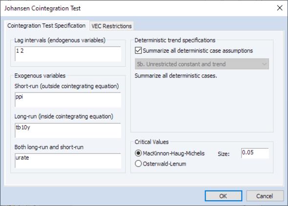
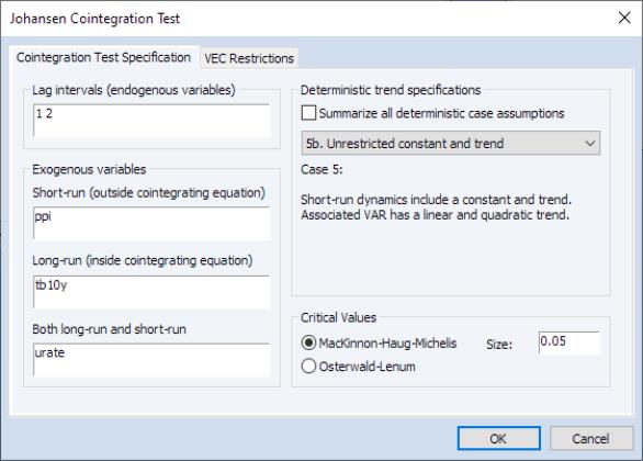
Notice in our example that we've included all 3 types of exogenous variables. PPI is included among short-run exogenous variables; TB10Y is included among long-run exogenous variables; whereas URATE is estimated simultaneously among short- and long-run regressors.
Adding exogenous variables in the cointegration test requires some thought about how the variables affect the level and trend of the endogenous variables
Keep in mind that the exogenous variables entered in the test dialog refer to short-run variables added to the VEC difference specification
Equation (45.41). This treatment is in contrast to that of the built-in deterministic trends which are specified in terms of the levels equation. For example, one of the most commonly added exogenous variables are seasonal dummy variables. Note, however, that if you include 0–1 seasonal dummy variables in the test specification, this will affect both the mean and the trend of the level series

. To handle this problem, Johansen (1995, page 84) suggests using centered (orthogonalized) seasonal dummy variables, which shift the mean without contributing to the trend. Centered seasonal dummy variables for quarterly and monthly series can be generated by the commands:
series d_q = @seas(q) - 1/4
series d_m = @seas(m) - 1/12
for quarter

and month

, respectively.
Deterministic Trends
Your series may have nonzero means and deterministic trends as well as stochastic trends. Similarly, the cointegrating equations may have intercepts and deterministic trends. The asymptotic distribution of the LR test statistic for cointegration does not have the usual

distribution and depends on the assumptions made with respect to deterministic trends. To carry out the test, you need to make an assumption regarding the trend underlying your data.
The empirical literature has centered around several commonly specified scenarios involving deterministic terms:
• Case 1: No deterministics.
• Case 2: Restricted constant, so that the constant is restricted to the cointegrating space and does not appear in the transitory space. The cointegrating mean is non-zero and the cointegrating equation restriction ensures that no linear trends exist in the corresponding VAR.
• Case 3: Unrestricted constant, so that the constant appears in the transitory space but does not appear in the cointegrating space.
The model has no deterministics in the cointegrating space, and exhibits a linear trend in the VAR representation.
• Case 3 (JHJ): Unrestricted constant in both the transitory and the cointegrating space so that the specification has a non-zero mean in the cointegrating relations, and has a linear trend in the corresponding VAR.
• Case 4: Unrestricted constant and restricted trend so that a constant appears in the transitory space but does not appear in the cointegrating space, and the trend term appears only in the cointegrating space.
This model has a linear trend in the cointegrating relations, and has a linear trend in the corresponding VAR representation.
• Case 4 (JHJ): Unrestricted constant and restricted trend so that the constant appears in both the transitory space and the cointegrating space, while the trend term appears only in the cointegrating space.
The model has a non-zero mean and non-zero trend in the cointegrating relations, and has a linear trend in the corresponding VAR formulation.
• Case 5: Unrestricted constant and trend, so that the constant and trend appears in the transitory space.
The model has a non-zero mean and non-zero trend in the cointegrating relations, and has a quadratic trend in the corresponding VAR.
• Case 5 (JHJ): Unrestricted constant and trend, the constant and trend appear in both the transitory and cointegrating spaces.
The model has a non-zero mean and non-zero trend in the cointegrating relations, and has a quadratic trend in the corresponding VAR formulation.
You may use the dropdown menu in the d Specification section to choose one of these assumptions. Alternately, you may select the checkbox to construct a summary of cointegration tests for all of the deterministic specifications.
For a full discussion of VECM deterministic specifications, see the discussion in
“VECMs with Deterministics”.
Critical Values
The asymptotic distribution of the LR test statistic for cointegration does not have the usual

distribution and depends on the assumptions made with respect to deterministic trends.
By default, EViews will compute the critical values for the test using MacKinnon-Haug-Michelis (MHM, 1999) p-values. By default, EViews will compute the critical values for the test using MHM, but you may elect instead to report the Osterwald-Lenum (OL, 1992) at the 5% and 1% levels by changing the radio button selection from to .
Critical values are available for up to

series.
Note also that while the critical values reported by EViews account for the presence of popular deterministic specifications, they do not account for the presence of general exogenous variables.
Examples of Johansen Cointegration Tests
We may perform Johansen cointegration testing and rank determination using the example workfile “var1.WF1”, located under the
“Vector Autoregression (VAR) Models” folder. This is a workfile with a number of classic macroeconomic variables including gross domestic product, various measure of money supply, treasury bills of different maturations, industrial production, producer price index, the unemployment.
Single Cointegration Test
We may carry out a Johansen cointegration test to determine the cointegrating rank. This test is available from a group window using , or from an estimated VAR object window using
Suppose we have open an estimated VAR object, click on and fill out the test dialog as follows:
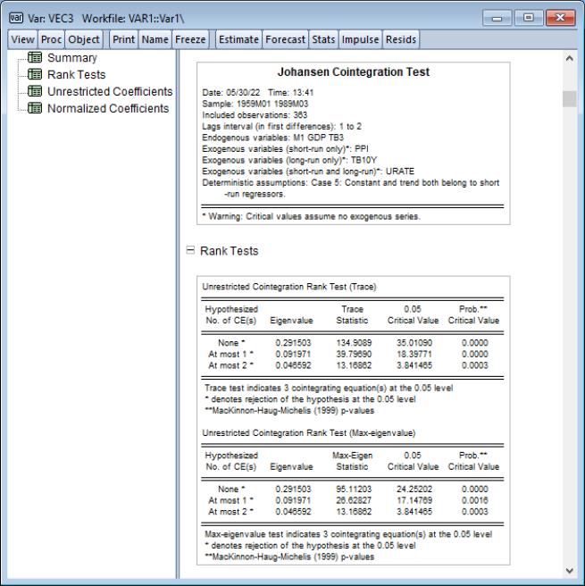
Click on to perform the test. The output is a spool object with 4 tables:
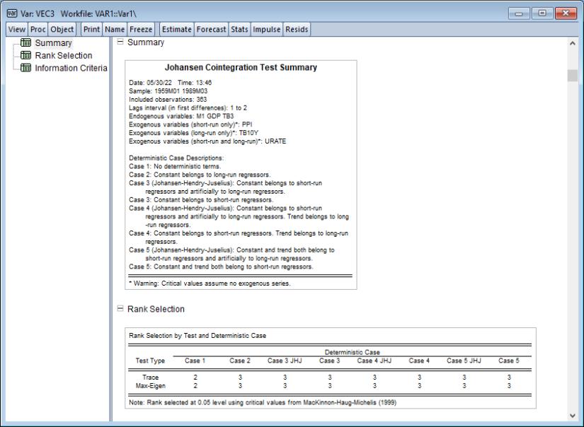
The first table is a of the estimation specifications under which the cointegration rank test is conducted.
Following the summary is a table showing Johansen cointegration tests based on the trace and maximum eigenvalue statistics. The trace statistic reported in the first block tests the null hypothesis of at most

cointegrating relations against the alternative of

cointegrating relations, where

is the number of endogenous variables. The maximum eigenvalue statistics tests the null hypothesis of

cointegrating relations against the alternative of

cointegrating relations.
In interpreting the results for these tests, we begin with the null hypothesis

. If a test rejects, increase the null

by one and repeat the test. The estimated cointegration rank is then the first (minimum)

for which the test fails to reject the null. In this case, we reject all three null hypotheses at conventional significance levels, and conclude that there are 3 cointegrating equations.
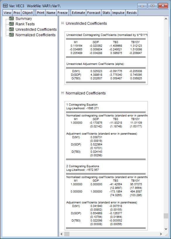
The next node contains the table which provides estimates of the cointegrating vector

and the adjustment parameters

. As is well known, the cointegrating vector

is not identified unless we provide an arbitrary normalization. This table reports estimates of

and

under the normalization

where

is defined in
Equation (45.22). Note that the transpose of

is reported in the table so that the first row is the first cointegrating vector, the second row is the second cointegrating vector, and so on.
The final node contains the table which reports estimates from a different normalization for each possible number of cointegrating relations. This alternative normalization expresses the first

variables as functions of the remaining

variables in the system. Asymptotic standard errors are reported in parentheses for the parameters that are identified.
Rank Tests Summary
It is possible to conduct a battery of rank tests for each of the deterministic assumptions that are available for estimation. To do this, proceed from the previous example and click on to once again bring up the testing dialog.
This time, click on and hit .
The top portion of the spool output shows the test settings and assumptions, along with the rank selection results broken down by test type and deterministic case:
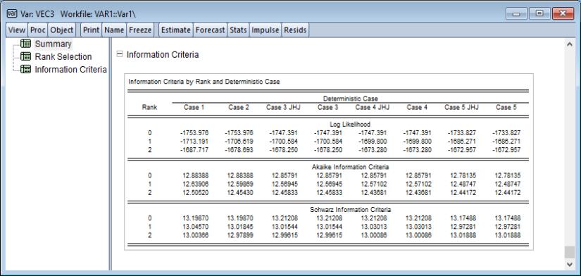
The remainder of the output shows the information criteria broken down by rank and deterministic case:
 . Accordingly, we consider formal methods for determining the cointegrating rank using Johansen cointegration tests.
 . Accordingly, we consider formal methods for determining the cointegrating rank using Johansen cointegration tests.
 endogenous variables and no deterministic terms,
 has rank
  for
for  , then there exist
  matrices
  and
and  each with rank
  such that
  .
. :
:  versus
  :
: 
 :
:  versus
  :
: 

 denotes the maximized value of the Gaussian likelihood function for cointegration rank
  , and
, and  are the eigenvalues associated with the relevant symmetric matrix given in
 are nonstandard and are given by:
 and
and  are respectively the trace and maximum eigenvalue of the matrix
 is the
  -dimensional standard Wiener process.
  and
and  are commonly referred to as the
  . If a test rejects, increase the null
  by one and repeat the test. The estimated cointegration rank is then the first (minimum)
  for which the test fails to reject the null.
 and
and  instead of
  and
and  . (
. (
 matrix has full rank (
 ). This apparent contradiction may be the result of low power of the cointegration tests, stemming perhaps from a small sample size or serving as an indication of specification error.
 on
on  ,
,  , and any other exogenous variables that you have specified. Note that in terms of the level series
  the largest lag is 3. To run a cointegration test with one lag in the
  . To handle this problem, Johansen (1995, page 84) suggests using centered (orthogonalized) seasonal dummy variables, which shift the mean without contributing to the trend. Centered seasonal dummy variables for quarterly and monthly series can be generated by the commands:
 and month
  , respectively.
 distribution and depends on the assumptions made with respect to deterministic trends. To carry out the test, you need to make an assumption regarding the trend underlying your data.
 distribution and depends on the assumptions made with respect to deterministic trends.
 series.
 cointegrating relations against the alternative of
  cointegrating relations, where
  is the number of endogenous variables. The maximum eigenvalue statistics tests the null hypothesis of
  cointegrating relations against the alternative of
  cointegrating relations.
 . If a test rejects, increase the null
  by one and repeat the test. The estimated cointegration rank is then the first (minimum)
  for which the test fails to reject the null. In this case, we reject all three null hypotheses at conventional significance levels, and conclude that there are 3 cointegrating equations.
 and the adjustment parameters
  . As is well known, the cointegrating vector
  is not identified unless we provide an arbitrary normalization. This table reports estimates of
  and
and  under the normalization
  where
where  is defined in
 is reported in the table so that the first row is the first cointegrating vector, the second row is the second cointegrating vector, and so on.
 variables as functions of the remaining
  variables in the system. Asymptotic standard errors are reported in parentheses for the parameters that are identified.