Estimating VEC Models in EViews
Estimation of VEC model in EViews is a special case of estimation in a var object. From the main application menu of an existing var object, click on the button to open the estimation dialog. Alternately, you may create a new VAR object by selecting Object/New Object... group, then selecting . Once the dialog appears, select in the dropdown menu to display the VEC estimation dialog:
Once you have filled the in the dialog, simply click OK to estimate the VEC. Estimation of a VEC model is carried out in two steps. In the first step, we estimate the cointegrating relations from the Johansen procedure as used in the cointegration test. We then construct the error correction terms from the estimated cointegrating relations and estimate a VAR in first differences including the error correction terms as regressors.
There are three tabs in the dialog: , , and . We discuss each of these tabs in turn.
Basic Specification
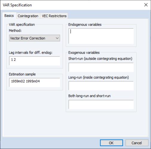
In the Basics tab, you will provide the usual information about the , ,and lists of different types of :
• Importantly, in contrast to the standard VAR case, the specification refers to lags of the first difference terms in the conditional EC representation of the VEC. For example, the lag specification “1 1” will include lagged first difference terms on the right-hand side of the VEC. Rewritten in levels, this VEC is a restricted VAR with two lags. To estimate a VEC with no lagged first difference terms, specify the lag as “0 0”
• The section allows you to specify exogenous variables that are not included in the standard in-built deterministic trend cases. This convention means that the constant and linear trend term should not be included in the Exogenous variables edit boxes. The constant and trend specification for VECs should be specified using the dropdown menu in the Cointegration tab.
You should enter any other variables in the edit field corresponding to whether they appear in the , , or lists of variables.
Note that the exogenous variables entered in the VEC estimation dialog refer to short-run variables added to the VEC difference specification
Equation (45.41). This treatment is in contrast to that of built-in deterministics in VEC estimation and of exogenous variables when estimating a VAR, where the specified variables are entered into the levels equation
Equation (45.1). (See
“Exogenous Variables in VECMs” for further discussion.)
Cointegration Options
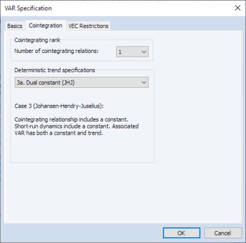
Important options related to cointegration can be accessed by clicking on the Cointegration tab:
• A fundamental prerequisite of VECM estimation is
a priori knowledge of the number of cointegrating relations

. You may use the dropdown menu to select the appropriate (see
“Johansen Cointegration Test” for determination of cointegrating rank).
Note that as you make a selection in the dropdown, the text below will change to give you a more detailed description of the assumptions underlying the choice.
VEC Restrictions
Since the cointegrating vector

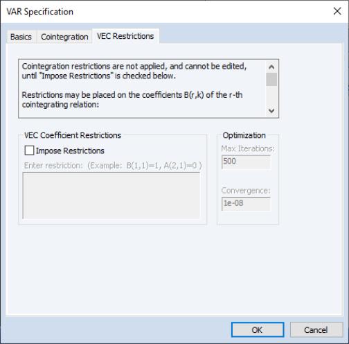
is not fully identified, EViews applies standard normalizations to identify the remaining coefficients. Alternately, you may wish to impose your own identifying restrictions when performing estimation. Restrictions may be imposed on the cointegrating vector (elements of the

matrix) and/or on the adjustment coefficients (elements of the

matrix).
To impose restrictions in estimation, click on the tab to display the restrictions dialog. You will enter your restrictions in the edit box that appears when you check the box:
“Specifying VEC Restrictions” describes the syntax for specifying these restrictions in greater detail.
Specifying VEC Restrictions
Restrictions can be imposed on the cointegrating vector (elements of the

matrix) and/or on the adjustment coefficients (elements of the

matrix).
Restrictions on the Cointegrating Vector
To impose restrictions on the cointegrating vector

, you must refer to the (
i,
j)-th element of the
transpose of the

matrix by
B(i,j). The
i-th cointegrating relation has the representation:
B(i,1)*y1 + B(i,2)*y2 + ... + B(i,k)*yk
where y1, y2, ... are the (lagged) endogenous variable. Then, if you want to impose the restriction that the coefficient on y1 for the second cointegrating equation is 1, you would type the following in the edit box:
B(2,1) = 1
You can impose multiple restrictions by separating each restriction with a comma on the same line or typing each restriction on a separate line. For example, if you want to impose the restriction that the coefficients on y1 for the first and second cointegrating equations are 1, you would type:
B(1,1) = 1
B(2,1) = 1
Currently
all restrictions must be linear (or more precisely affine) in the elements of the  matrix
. So for example
B(1,1) * B(2,1) = 1
will return a syntax error.
Restrictions on the Adjustment Coefficients
To impose restrictions on the adjustment coefficients, you must refer to the (
i,
j)-th elements of the

matrix by
A(i,j). The error correction terms in the
i-th VEC equation will have the representation:
A(i,1)*CointEq1 + A(i,2)*CointEq2 + ... + A(i,r)*CointEqr
Restrictions on the adjustment coefficients are currently limited to linear homogeneous restrictions so that you must be able to write your restriction as
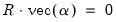
, where

is a known

matrix. This condition implies, for example, that the restriction,
A(1,1) = A(2,1)
is valid but:
A(1,1) = 1
will return a restriction syntax error.
One restriction of particular interest is whether the
i-th row of the

matrix is all zero. If this is the case, then the
i-th endogenous variable is said to be
weakly exogenous with respect to the  parameters
. See Johansen (1995) for the definition and implications of weak exogeneity. For example, if we assume that there is only one cointegrating relation in the VEC, to test whether the second endogenous variable is weakly exogenous with respect to

you would enter:
A(2,1) = 0
To impose multiple restrictions, you may either separate each restriction with a comma on the same line or type each restriction on a separate line. For example, to test whether the second endogenous variable is weakly exogenous with respect to

in a VEC with two cointegrating relations, you can type:
A(2,1) = 0
A(2,2) = 0
You may also impose restrictions on both
 and
and 
. However, the restrictions on

and

must be
independent. So for example,
A(1,1) = 0
B(1,1) = 1
is a valid restriction but:
A(1,1) = B(1,1)
will return a restriction syntax error.
Identifying Restrictions and Binding Restrictions
EViews will check to see whether the restrictions you provided identify all cointegrating vectors for each possible rank. The identification condition is checked numerically by the rank of the appropriate Jacobian matrix; see Boswijk (1995) for the technical details. Asymptotic standard errors for the estimated cointegrating parameters will be reported only if the restrictions identify the cointegrating vectors.
If the restrictions are binding, EViews will report the LR statistic to test the binding restrictions. The LR statistic is reported if the degrees of freedom of the asymptotic

-distribution is positive. Note that the restrictions can be binding even if they are not identifying, (
e.g. when you impose restrictions on the adjustment coefficients but not on the cointegrating vector).
Options for Restricted Estimation
Estimation of the restricted cointegrating vectors

and adjustment coefficients

generally involves an iterative process. The tab provides iteration control for the maximum number of iterations and the convergence criterion. EViews estimates the restricted

and

using the switching algorithm as described in Boswijk (1995). Each step of the algorithm is guaranteed to increase the likelihood and the algorithm should eventually converge (though convergence may be to a local rather than a global optimum). You may need to increase the number of iterations in case you are having difficulty achieving convergence at the default settings.
Once you have filled the dialog, simply click OK to estimate the VEC. Estimation of a VEC model is carried out in two steps. In the first step, we estimate the cointegrating relations from the Johansen procedure as used in the cointegration test. We then construct the error correction terms from the estimated cointegrating relations and estimate a VAR in first differences including the error correction terms as regressors.