How to Estimate an Elastic Net Specification in EViews
To estimate a elastic net (Enet) specification in EViews you must first create an equation object. You may select or from the main menu, or enter the keyword equation in the command window. Next, select in the drop-down menu. Alternately, entering the keyword enet in the command window will create a new equation object and automatically set the estimation method.
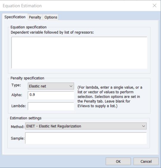
EViews will open a dialog showing settings appropriate an elastic net specification:
The Specification Tab
The tab displays settings for the variables in the equation specification, basic penalty definition, and the estimation sample. As the should be familiar, we focus our attention on the first two sections
Equation Specification
You should enter the dependent variable followed by a list of regressor series or group objects in the edit field. The special “C” regressor variable keyword may be used to include an unpenalized intercept in the specification.
Note that PDL and ARMA terms are not permitted in ENET estimation.
If you wish to specify individual regressors with penalty weight

in
Equation (37.1), or wish to place inequality restrictions on the coefficient values, you may do so using special expressions of the form:
@vw(series_name, weight_value)
or
@vw(series_name[, wgt=weight_value, cmin=coef_min, cmax=coef_max])
where weight_value is a non-negative value, coef_min is a non-positive minimum coefficient value, and coef_max is a non-negative maximum coefficient value.
There are two forms of the special expression. In the specialized abbreviated form, you specify the variable name followed by the penalty weight value. In the more general form, you may specify the variable name followed by one or more keyword expressions in arbitrary order, with the “wgt=” argument specifying the penalty weight, “cmin=” giving a non-positive minimum coefficient value, and “cmax=” providing a non-negative maximum coefficient value.
As an example,
y c x @vw(z, cmax=10, wgt=0.5) @vw(w, 0.0)
specifies an elastic net model with dependent variable Y, unpenalized intercept C, penalized variable X with default weight

, Z with individual weight

and maximum value of 10, and unpenalized W.
When specifying individual regressor behavior using @vw, keep in mind that:
• The intercept variable “C” is always non-penalized so that it has an implicit weight of 0.0.
• Individual penalty weights may also be specified using a vector in the edit field on the dialog page (or using the command estimation option “lambdawgt=vector_name”). If the vector weights are specified and individual weights are specified using the @vw keyword, the vector weights will be applied first, followed by the individual variable weights.
• Individual coefficient limit values may also be specified using vectors in the and edit fields on the dialog page (or the command estimation options “coefmin=vector_name” and “coefmax =vector_name”). If vector coefficient limits are specified and individual regressor limits are specified using the @vw keyword, the vector limits will be applied first, followed by the individual limits weights.
EViews will normalize the individual penalty weights so that they sum to the number of non-zero weights:

where

is the number of non-zero

.
Parameter Specification
The section may be used to specify the penalty component:
Type and Alpha
The drop-down menu and edit field specify the mixing parameter. You may use the to choose between the default estimator, or the or presets.
• For the estimator, you will be prompted to specify a value for the mixing parameter

in the edit field,

. By default,

is set to 0.9.
EViews does not allow you to specify multiple values of the

parameter.
• For the preset, the mixing parameter

is fixed at 1.0.
• For the preset, the mixing parameter

is fixed at 0.0.
Bear in mind that the preset corresponds to a specialized ridge regression estimator that employs a closed-form solution. The penalty parameters should be specified in the traditional parameterization

, and not in the elastic net parameterization,

(see
“The Mixing Parameter” for discussion).
If you wish to estimate ridge regression as a special case of elastic net you should specify your as and enter “0” for

, and specify the parameter

in using the elastic net parameterization.
Lambda
The edit field controls the overall penalty parameter

. You may enter a single value, multiple values in the form of a list of values and/or vector objects, or you may leave the edit field blank to have EViews automatically determine a list of values.
If there are multiple

values, EViews will sort the values from high-to-low, and perform path estimation using values from the higher

estimates as “warm” starting values for the next lower

. EViews will perform cross-validation model selection to identify a “best”

from among the specified values.
Additional options for the specification of

values and options controlling cross-validation model selection are specified in the tab of the dialog.
The Penalty Tab
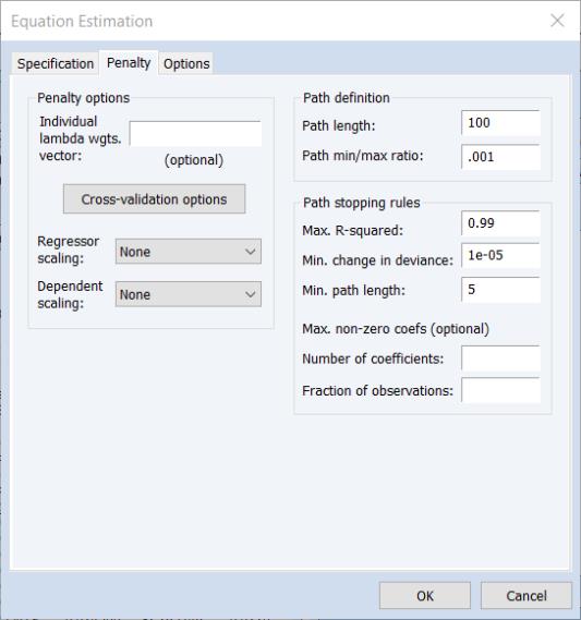
Additional options related to the computation of the coefficient penalty are specified in the tab of the dialog:
There are three sections in this dialog: a section which contains options that affect the penalty calculations, a section which controls the automatic determination of a list of penalty values, and a section which controls the computation of estimates along the

-path.
Penalty Options
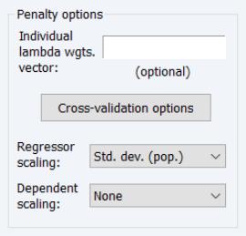
The section provides settings related to the computation and selection of penalty values.
Individual Penalty Weights
Individual penalty weights

may be specified using a vector in the workfile by entering the vector name in the edit field. The vector containing non-negative values should be sized to match the number of coefficients in the specification.
If vector weights are specified here, and individual weights are specified in the dialog page using the
@vw keyword (
“Equation Specification”), the vector weights will be applied first, followed by the individual variable weights.
Cross-validation Options
There is a button that is enabled if you have specified multiple

values in the tab. These options provide settings for controlling the cross-validation model selection procedure which computes an optimal value of

. See
“Cross-validation Settings” for details.
Variable Scaling
The and drop-down menus control settings for the automatic scaling of your data. You may choose between: , , , , , and scaling:
• The and scales specify whether to use the biased population (division by

) or unbiased sample (division by

) estimates of the data variance.
• The setting employs the

-norm divided by

,
• The setting uses the

-norm divided by

.
• The setting corresponds to using the range of the data as the scale.
By default, the regressors will be scaled using the square root of the biased estimator of the data variance: , and the dependent variable will be unscaled.
The choice of data scaling can be an important one. Regressor scaling will generally alter the relative values of estimated coefficients, and dependent variable scaling will affect relative coefficient values in some specifications (see
“Data scaling” for discussion).
Further, note that:
• If you specify automatic dependent variable scaling, EViews will scale user-provided, original scale

values to account for the automatic adjustment. EViews determined

path values will be obtained using the scaled data,. All
 values will be reported on the original scale
.
• When you specify automatic dependent or regressor scaling, EViews will estimate the elastic net model using the scaled data as specified, and the coefficient results will be reported in the original scale.
Automatic Path Definition
When the text box on the main tab is left blank, EViews will automatically determine a grid of

values using the approach outlined in
“Automatic Lambda Grid”.
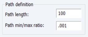
Two options for the automatic construction of this path are contained in the section:
First, is the maximum number of

values to specify along the path. The default length of the path is 100.
Second, the is the ratio of the largest value of

to the smallest value of

along the path. The largest value is determined by using the data to compute the smallest

penalty for which all of the estimated coefficients are 0. (For ridge regression specifications, coefficients are not easily pushed to zero, so we arbitrarily use an elastic net model with

to determine this penalty.) The resulting

will be the largest value of

considered. The smallest value is

times the value of this parameter. The default value is 0.001.
Path Stopping Rules
Given a set of

sorted from high to low,

, path estimation begins by estimating a model with

(the most penalized specification) and continuing to estimate successively less penalized models, using the results from the previous

as starting values. EViews will stop path estimation in the event that convergence is not achieved for a given

.
In practice, we may find that estimating additional models along the path provides little additional benefit in terms of model fit, or that there are excessively large numbers of non-zero estimated coefficients at the given

. In these cases, continuing along the path to estimate additional models at lower

offers little benefit at considerable computational cost.
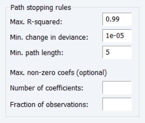
To account for this possibility, you may specify so that path estimation will stop when certain criteria are reached:
The first two options describe stopping rules associated with the model fit: path estimation will stop when the current model R-squared exceeds the value in the , or when thechange in the sum-of-squared residuals (deviance) between the prior

model and the current

model is less than the value.
The option is a modifier to the path stopping rules, specifying the minimum number of path lambda to estimate before applying any stopping rules.
The remaining optional edit fields allow you to stop the path estimation when the number of non-zero coefficients becomes large. You may specify the limit on the number of coefficients as an explicit value () or as a fraction of the number of observations in estimation (), or both. If specified, the coefficient restrictions are evaluated once the minimum path length requirement is satisfied.
The Options Tab
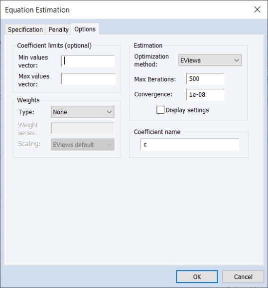
The tab contains the remaining estimation settings. There are four sections: , , , and .
Coefficient Limits
Coefficient minimum and maximum values may be specified using vectors or a scalar in the and edit fields.
The vectors containing the minimum non-positive and the maximum non-negative values should be sized to match the number of coefficients in the specification. Non-restricted coefficients are indicated using a NA in the corresponding vector element.
If vector coefficient limits are specified and individual regressor limits are specified using individual variables with the
@vw keyword in the
Specification page (see
“Equation Specification”), the vector limits will be applied first, followed by the individual limits.
Weights
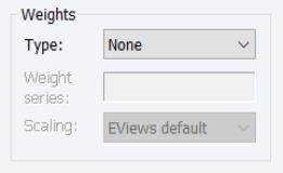
The familiar section allows you to specify individual estimation weights.
The dropdown menu is used to specify the form of the data in the specified weight series: , , , , or . If you select a other than , EViews will prompt you to provide a weight series name. The dropdown menu allows you to specify a scale to apply to the values in the weight series. By default EViews scales the weights so the square roots sum to

.
See
“Weighted Least Squares” of
User’s Guide I for further discussion.
Estimation
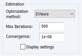
The section offers settings for controlling iterative estimation.
Optimization Method
For the ridge regression method, the iterative optimization options will be disabled since EViews estimates the coefficients using the closed form estimator.
For elastic net and Lasso estimation, the allows you to choose between the , , and methods. Discussion of the choice requires a bit of background.
Briefly, iterative estimation of these penalized regression models is performed by EViews using the active-set cyclical coordinate descent algorithm as described in detail by Hastie, Tibshirani, and Friedman (2010). Within this framework, the authors outline two approaches to cyclical coordinate descent which they term the naive and the covariance update methods.
When updating a coefficient using cyclical coordinate descent, the “naive” method computes the gradients of the loss with respect to an individual coefficient using the residuals computed at current residuals. Thus, a full update cycle with respect to all of the coefficients requires

residual updates; one full computation of the residuals as each coefficient is updated.
In contrast, the “covariance” method computes the inner product between all of the regressors and both the dependent variable and all regressors prior to beginning estimate. These moments are held for the remainder of the procedure and accessed in each coefficient update.
In most cases, the covariance method offers considerable efficiencies relative to the naive method as it does not require computation of residuals for each coefficient. Note however, that the covariance algorithm does require inner products for all regressors against all other regressors, the number of which increases with the square of the number of regressors. For very large numbers of coefficients, the computational and storage costs may make this approach impractical.
To balance these competing burdens, the setting offers a default estimation method which uses covariance updates if the number of variables is less than or equal to 200, and naive updates if the number of variables is greater than 200. You may use the , and settings to specify a method in place of this EViews default.
Iteration and Convergence
The and tolerance edit fields control those two aspects of estimation. The option is self-explanatory. The setting needs a bit of discussion.
Convergence for the EViews cyclical coordinate descent algorithm is defined in terms of changes in coefficients. We follow Hastie, Tibshirani, and Friedman (2010) in defining the scaled coefficient difference for a coefficient update as the squared change in the coefficient divided by the average of the squared values of the corresponding regressor. Convergence is achieved when the maximum of the scaled coefficient differences falls below the specified value.
Coefficient Name
Enter the name of a coefficient vector to replace the default “C” used in estimation. The Coef object will be created and sized, or resized as needed.

 in
Equation (37.1), or wish to place inequality restrictions on the coefficient values, you may do so using special expressions of the form:
 , Z with individual weight
  and maximum value of 10, and unpenalized W.
  where
where  is the number of non-zero
  .
.
 in the Alpha edit field,
  . By default,
  is set to 0.9.
 parameter.
 is fixed at 1.0.
 is fixed at 0.0.
  , and not in the elastic net parameterization,
  (see
“The Mixing Parameter” for discussion).
 , and specify the parameter
  in using the elastic net parameterization.
 . You may enter a single value, multiple values in the form of a list of values and/or vector objects, or you may leave the edit field blank to have EViews automatically determine a list of values.
 values, EViews will sort the values from high-to-low, and perform path estimation using values from the higher
  estimates as “warm” starting values for the next lower
  . EViews will perform cross-validation model selection to identify a “best”
  from among the specified values.
  values and options controlling cross-validation model selection are specified in the Penalty tab of the dialog.
 -path.
 may be specified using a vector in the workfile by entering the vector name in the Individual lambda wgts. vector edit field. The vector containing non-negative values should be sized to match the number of coefficients in the specification.
  values in the Specification tab. These options provide settings for controlling the cross-validation model selection procedure which computes an optimal value of
  . See
“Cross-validation Settings” for details.
 ) or unbiased sample (division by
  ) estimates of the data variance.
  -norm divided by
  ,
,  -norm divided by
  .
.  values to account for the automatic adjustment. EViews determined
  path values will be obtained using the scaled data,. All
  values will be reported on the original scale.
 values using the approach outlined in
“Automatic Lambda Grid”.
 values to specify along the path. The default length of the path is 100.
 to the smallest value of
  along the path. The largest value is determined by using the data to compute the smallest
  penalty for which all of the estimated coefficients are 0. (For ridge regression specifications, coefficients are not easily pushed to zero, so we arbitrarily use an elastic net model with
  to determine this penalty.) The resulting
  will be the largest value of
  considered. The smallest value is
  times the value of this parameter. The default value is 0.001.
 sorted from high to low,
  , path estimation begins by estimating a model with
  (the most penalized specification) and continuing to estimate successively less penalized models, using the results from the previous
  as starting values. EViews will stop path estimation in the event that convergence is not achieved for a given
  .
. . In these cases, continuing along the path to estimate additional models at lower
  offers little benefit at considerable computational cost.
 model and the current
  model is less than the Min. change in deviance value.
 .
.
 residual updates; one full computation of the residuals as each coefficient is updated.