Panel Equation Testing
Omitted Variables Test
You may perform an F-test of the joint significance of variables that are presently omitted from a panel or pool equation estimated by list. Select and in the resulting dialog, enter the names of the variables you wish to add to the default specification. If estimating in a pool setting, you should enter the desired pool or ordinary series in the appropriate edit box (common, cross-section specific, period specific).
When you click on , EViews will first estimate the unrestricted specification, then form the usual F-test, and will display both the test results as well as the results from the unrestricted specification in the equation or pool window.
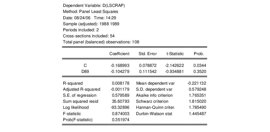
Adapting Example 10.6 from Wooldridge (2002, p. 282) slightly, we may first estimate a pooled sample equation for a model of the effect of job training grants on LSCRAP using first differencing. The restricted set of explanatory variables includes a constant and D89. The results from the restricted estimator are given by:
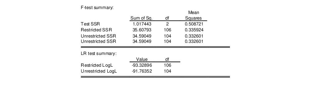
We wish to test the significance of the first differences of the omitted job training grant variables GRANT and GRANT_1. Click on and type “D(GRANT)” and “D(GRANT_1)” to enter the two variables in differences. Click on to display the omitted variables test results.
The top portion of the results contains a brief description of the test, the test statistic values, and the associated significance levels:
Here, the test statistics do not reject, at conventional significance levels, the null hypothesis that D(GRANT) and D(GRANT_1) are jointly irrelevant.
The remainder of the results shows summary information and the test equation estimated under the unrestricted alternative:
Note that if appropriate, the alternative specification will be estimated using the cross-section or period GLS weights obtained from the restricted specification. If these weights were not saved with the restricted specification and are not available, you may first be asked to reestimate the original specification.
Redundant Variables Test
You may perform an F-test of the joint significance of variables that are presently included in a panel or pool equation estimated by list. Select and in the resulting dialog, enter the names of the variables in the current specification that you wish to remove in the restricted model.
When you click on , EViews will estimate the restricted specification, form the usual F-test, and will display the test results and restricted estimates. Note that if appropriate, the alternative specification will be estimated using the cross-section or period GLS weights obtained from the unrestricted specification. If these weights were not saved with the specification and are not available, you may first be asked to reestimate the original specification.
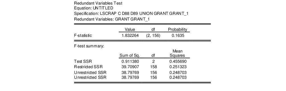
To illustrate the redundant variables test, consider Example 10.4 from Wooldridge (2002, p. 262), where we test for the redundancy of GRANT and GRANT_1 in a specification estimated with cross-section random effects. The top portion of the unrestricted specification is given by:
.
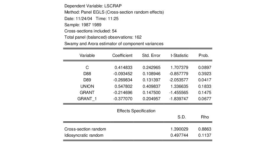
Note in particular that our unrestricted model is a random effects specification using Swamy and Arora estimators for the component variances, and that the estimates of the cross-section and idiosyncratic random effects standard deviations are 1.390 and 0.4978, respectively.
If we select the redundant variables test, and perform a joint test on GRANT and GRANT_1, EViews displays the test results in the top of the results window:
Here we see that the statistic value of 1.832 does not, at conventional significance levels, lead us to reject the null hypothesis that GRANT and GRANT_1 are redundant in the unrestricted specification.
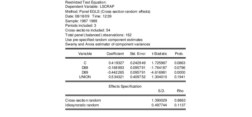
The restricted test equation results are depicted in the bottom portion of the window. Here we see the top portion of the results for the restricted equation:
The important thing to note is that the restricted specification removes the test variables GRANT and GRANT_1. Note further that the output indicates that we are using existing estimates of the random component variances (“Use pre-specified random component estimates”), and that the displayed results for the effects match those for the unrestricted specification.
Fixed Effects Testing
EViews provides built-in tools for testing the joint significance of the fixed effects estimates in least squares specifications. To test the significance of your effects you must first estimate the unrestricted specification that includes the effects of interest. Next, select . EViews will estimate the appropriate restricted specifications, and will display the test output as well as the results for the restricted specifications.
Note that where the unrestricted specification is a two-way fixed effects estimator, EViews will test the joint significance of all of the effects as well as the joint significance of the cross-section effects and the period effects separately.
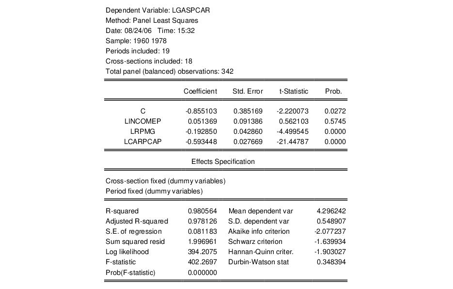
Let us consider Example 3.6.2 in Baltagi (2005), in which we estimate a two-way fixed effects model using data in “Gasoline.WF1”. The results for the unrestricted estimated gasoline demand equation are given by:
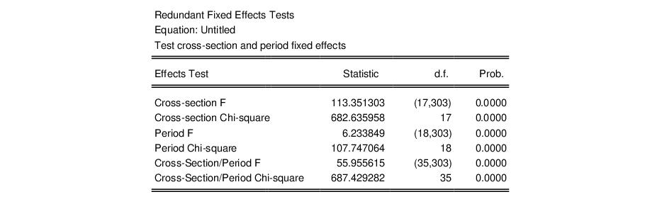
Note that the specification has both cross-section and period fixed effects. When you select the fixed effect test from the equation menu, EViews estimates three restricted specifications: one with period fixed effects only, one with cross-section fixed effects only, and one with only a common intercept. The test results are displayed at the top of the results window:
Notice that there are three sets of tests. The first set consists of two tests (“Cross-section F” and “Cross-section Chi-square”) that evaluate the joint significance of the cross-section effects using sums-of-squares (F-test) and the likelihood function (Chi-square test). The corresponding restricted specification is one in which there are period effects only. The two statistic values (113.35 and 682.64) and the associated p-values strongly reject the null that the cross-section effects are redundant.
The next two tests evaluate the significance of the period dummies in the unrestricted model against a restricted specification in which there are cross-section effects only. Both forms of the statistic strongly reject the null of no period effects.
The remaining results evaluate the joint significance of all of the effects, respectively. Both of the test statistics reject the restricted model in which there is only a single intercept.
Below the test statistic results, EViews displays the results for the test equations. In this example, there are three distinct restricted equations so EViews shows three sets of estimates.
Lastly, note that this test statistic is not currently available for instrumental variables and GMM specifications.
Hausman Test for Correlated Random Effects
A central assumption in random effects estimation is the assumption that the random effects are uncorrelated with the explanatory variables. One common method for testing this assumption is to employ a Hausman (1978) test to compare the fixed and random effects estimates of coefficients (for discussion see, for example Wooldridge 2002, p. 288), and Baltagi 2005, p. 66).
To perform the Hausman test, you must first estimate a model with your random effects specification. Next, select . EViews will automatically estimate the corresponding fixed effects specifications, compute the test statistics, and display the results and auxiliary equations.
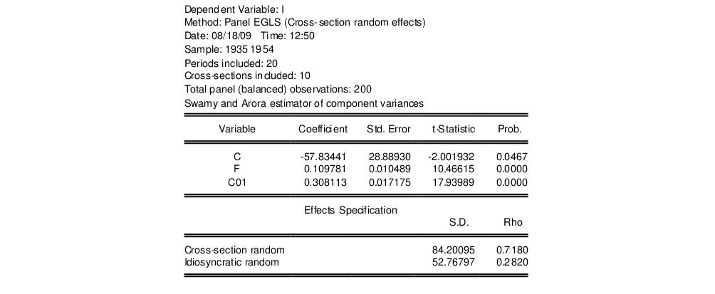
For example, Baltagi (2005) considers an example of Hausman testing (Example 1, p. 70), in which the results for a Swamy-Arora random effects estimator for the Grunfeld data (“Grunfeld_baltagi_panel.WF1”) are compared with those obtained from the corresponding fixed effects estimator. To perform this test we must first estimate a random effects estimator, obtaining the results:
Next we select the Hausman test from the equation menu by clicking on . EViews estimates the corresponding fixed effects estimator, evaluates the test, and displays the results in the equation window. If the original specification is a two-way random effects model, EViews will test the two sets of effects separately as well as jointly.
There are three parts to the output. The top portion describes the test statistic and provides a summary of the results. Here we have:
The statistic provides little evidence against the null hypothesis that there is no misspecification.
The next portion of output provides additional test detail, showing the coefficient estimates from both the random and fixed effects estimators, along with the variance of the difference and associated p-values for the hypothesis that there is no difference. Note that in some cases, the estimated variances can be negative so that the probabilities cannot be computed.
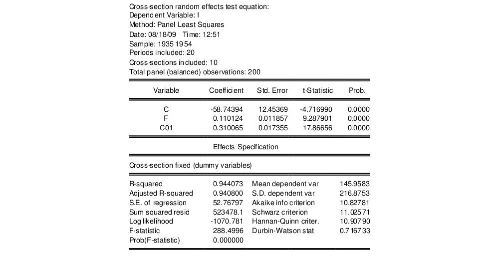
The bottom portion of the output contains the results from the corresponding fixed effects estimation:
In some cases, EViews will automatically drop non-varying variables in order to construct the test statistic. These dropped variables will be indicated in this latter estimation output.
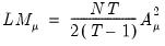
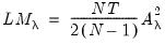
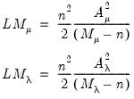
LM Tests for Random Effects
Testing for the existence of cross-section (individual) and time effects is important in panel and pool regression settings since accounting for the presence of these effects is necessary for correct specification of the regression and proper inference. As a result, a large number of effects tests have been considered in the literature. See, for example, the survey by Baltagi (2008).
EViews offers testing for individual and time effects using both F-statistic (likelihood ratio) and Lagrange multiplier (LM) tests. The follow discussion describes LM testing for random effects (the F-statistic tests for fixed effects are described elsewhere in this manual).
The most popular random effects test is the Breusch-Pagan (1980) LM test. Honda (1985) derives component LM tests with one-sided alternatives, obtaining a uniformly most powerful (UMP) test statistic. Moulton and Randolph (1989) propose a standardized version of the Honda test that has improved asymptotic size. King and Wu (1997) introduce a locally mean most powerful (LMMP) one-sided LM test. In addition, Baltagi and Li (1992), Baltagi, Chang and Li (1999) extend the Breusch-Pagan, Honda, and King and Wu approaches to unbalanced designs.
The EViews panel effects (PE) test view computes the following LM tests:
• Conventional LM (Breusch-Pagan, 1980)
• Uniformly most powerful LM (Honda, 1985)
• Standardized LM (Moulton and Randolph, 1989; Honda, 1991; Baltagi et al., 1999)
• Locally mean most powerful (LMMP) (King and Wu, 1997)
• Gourieroux, Holly, and Monfort (1982)
All of these tests may be computed from estimated regressions for equation objects in a panel structured workfile, or estimated pool objects in a non-panel workfile. Note that EViews offers these tests for equations estimated using both regression and instrumental variables so long as the equations are free of estimated effects, AR terms, and GLS weighting, despite the fact that these LM tests are not, strictly speaking, applicable in the instrumental variables case. One should employ appropriate caution in the use of such results in this setting.
Background
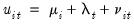
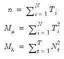
Our discussion follows closely the survey by Baltagi (2008). We consider two-way error components disturbances:
 | (55.5) |
for cross-sections

and periods
where

are unobservable individual effects,

are unobservable time effects, and

is the remaining idiosyncratic disturbance.
The LM tests are derived under the assumption that the unobserved individual effects are distributed as independent

, the unobservable time effects are independent

, and the idiosyncratic disturbances are independent

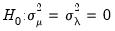
. The null hypotheses to be tested are: no individual effects (

); no time effects (

); and no individual and time effects (
).
For the remaining discussion, it will be useful to write the component specification in stacked matrix form. Let
. Then, define the cross-section residual vector
and stacked residuals
, we have
 | (55.6) |
where

is a
matrix of cross-section dummies,

is a
matrix of period dummies, and

is defined analogously to

.
For a balanced panel,
and
, where

is a

-dimensional identity matrix and

a

-dimensional unit vector. We also have
and
, for

a

matrix of ones.
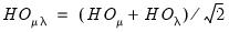
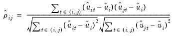
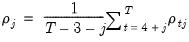
Breusch-Pagan Two-Sided Test
Breusch and Pagan (1980) derive the two-sided LM test for error components in balanced panels. Define
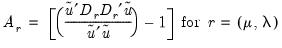 | (55.7) |
where

are the residuals obtained from the restricted model. Then defining
 | (55.8) |
and
 | (55.9) |
we obtain the LM statistic for testing

:
which is distributed as a

under the null. To test

and

, we may use

and

respectively, both of which are distributed as a

under corresponding null.
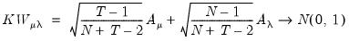
Baltagi and Li (1990) derived corresponding statistics for unbalanced samples:
 | (55.10) |
where
 | (55.11) |
which simplifies for the balanced case where

and

.
Honda UMP One-Sided Test
One shortcoming of the Breusch-Pagan test is that it assumes that the alternative hypothesis is two-sided even though the variance components cannot be negative.
Honda(1985) derives a uniformly most powerful

statistic for

against a one-sided

:
 | (55.12) |
Similarly, for the one-sided test of

against

we have:
 | (55.13) |
Note that both of these statistics are the square roots of the corresponding Breusch-Pagan LM statistics.
Honda’s statistics can be generalized to the unbalanced case yielding square roots of the unbalanced Breusch-Pagan LM statistics:
 | (55.14) |
Honda does not derive a uniformly most powerful statistic

against the one-sided alternative, but does suggest a “
handy” one-sided test statistic:
 | (55.15) |
which also converges to a

.
King and Wu
King and Wu (1997) propose locally mean most powerful (LMMP) one-sided test statistics

and

for

against a one-sided

and for

against

. These two statistics are identical to the corresponding Honda UMP statistics.
Baltagi, Chang, and Li (1992) derive the corresponding LMMP test for

against the one-sided alternative:
 | (55.16) |
and Baltagi, Chang, and Li (1999) obtain results for unbalanced case:
 | (55.17) |
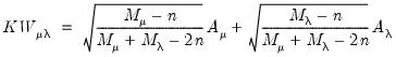
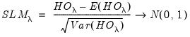
Standardized LM Tests
Moulton and Randolph (1989) showed that the asymptotic approximation for the one-sided statistics can be poor when the number of regressors is large or the inter-correlation of regressors is high. Alternatively, they propose a standardized one-sided LM (SLM) statistic which centers and scales the statistic so that its mean is zero and its variance is one.
For

against a one-sided

, they show that the standardized Honda (or King-Wu statistic) is given by:
 | (55.18) |
Expressions for the expected value and variance may be found in Moulton and Randolph (1989) and Baltagi (2008).
The one-sided statistic

for

against a one-sided

is defined analogously:
 | (55.19) |
For the two-way model, Honda (1991) proposes a standardized Honda-type SLM test statistic, and Baltagi, Chang and Li (1999) describe a standardized King-Wu statistic. Under
, these SLM statistics are asymptotically distributed as

and their critical values should be more accurate than those of the corresponding unstandardized tests. See Baltagi, Chang, and Li (1999) and Baltagi (2008) for details.
Gourieroux, Holly, Monfort test
Gourieroux, Holly and Monfort (1982) and Baltagi, Chang and Li (1992) account for the possibility of negative estimates of the variance components with the following modification of the LM test under the null hypothesis

against the two-sided alternative
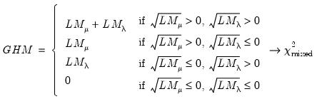 | (55.20) |
where

is a mixed

distribution with
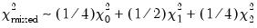
. The weights

,

and

are from Gourieroux
et al. (1982),

is zero with probability one, and

and

are asymptotically independent of each other.
Example
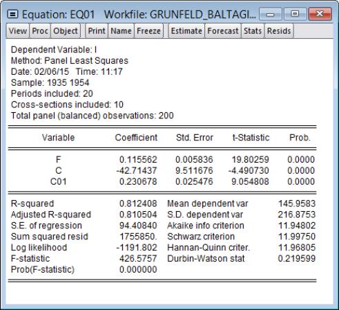
The LM test for random effects view implements Lagrange multiplier tests of individual or/and time effects based on the results of the pooling model. As an example we use the Grunfeld (1958) data which contains 10 large US manufacturing firms over 20 years (1935–1954), which is available in the workfile “Grunfeld_Baltagi_panel.wf1” in the “Working with Panel Data” folder in your “Example Files” directory.
Following Grunfeld (1958), we consider the following investment equation:
 | (55.21) |
where

denotes real gross investment for firm

in year

;

is the real value of the firm (share outstanding); and

is the real value of the capital stock. We estimate this model using ordinary pooled least squares on the specification:
i f c c01
and name our equation EQ01. The results are shown as below:
To test for the presence of individual and time effects in this model, we can click on menu item. The results of the LM tests are shown as below:
From the first column, we see that there is strong evidence that there are unaccounted for cross-section random effects in the pooled estimator residuals. All three of the cross-section tests have p-values well below conventional significance levels.
However, for testing time-specific effects, there is a marked difference between the results for the two-sided Breusch-Pagan and the one-sided tests, with the former suggesting the presence of effects, and the latter with negative values indicating that there are no time-effects. These data clearly show the benefits of using one-sided tests in an empirical setting.
Panel Cross-section Dependence Test
It is commonly assumed that disturbances in panel data models are cross-sectionally independent, especially when the cross-section dimension (

) is large. There is, however, considerable evidence that cross-sectional dependence is often present in panel regression settings.
Ignoring cross-sectional dependence in estimation can have serious consequences, with unaccounted for residual dependence resulting in estimator efficiency loss and invalid test statistics.
There are a variety of tests for cross-section dependence in the literature. EViews offers the following tests:
• Breusch-Pagan (1980) LM
• Pesaran (2004) scaled LM
• Baltagi, Feng, and Kao (2012) bias-corrected scaled LM
• Pesaran (2004) CD
These four tests may be computed from panel and pool equations estimated by least squares and instrumental variables. They may also be computed for series in a panel workfile.
Background
Following Pesaran (2004), suppose that we have a panel data model
 | (55.22) |
for
and
where

is a

-dimensional column vector of regressors,

are the corresponding cross-section specific vectors of parameters to be estimated. (Pesaran points out that while this specification has cross-section specific coefficients, the tests described below are also applicable to the more restrictive fixed and random effects models).
The general null hypothesis of no cross-section dependence may be stated in terms of the correlations between the disturbances in different cross-section units:
 | (55.23) |
For balanced samples,

is the product-moment correlation coefficients of the residuals
 | (55.24) |
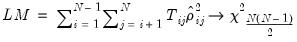
In the unbalanced case, Pesaran proposes use of the centered correlation coefficient
 | (55.25) |
where the notation

is used to indicate that we sum over the subset of

observations common to
i and
j, and the pairwise mean
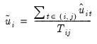 | (55.26) |
is used to adjust for the fact that the residuals in pairwise subsets are not necessarily mean zero.
(Note that in practice EViews always employs centered correlations as in
Equation (55.25) as this allows for estimation methods where the residuals are not constrained to have zero means in each cross-section. These results may differ from those that would have been obtained using the non-centered correlations in
Equation (55.24). EViews will provide a message informing you when non-zero means are found.)
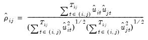
Breusch-Pagan LM
The most well-known cross-section dependence diagnostic is the Breusch-Pagan (1980) Lagrange Multiplier (LM) test statistic. In a seemingly unrelated regressions context, Breusch and Pagan show that under the null hypothesis in
Equation (55.23), a LM statistic for dependence is given by:
 | (55.27) |
where the

are the correlation coefficients obtained from the residuals of the model as described above. The asymptotic

distribution is obtained for

fixed as

for all

, and follows from a normality assumption on the errors.
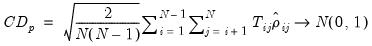
Pesaran Scaled LM
It is well known that the standard Breusch-Pagan LM test statistic is not appropriate for testing in large

settings. To address this shortcoming, Pesaran (2004) proposes a standardized version of the LM statistic
 | (55.28) |
which is asymptotically standard normal as first

and then

.
Pesaran notes one shortcoming of the scaled LM which is that

is not centered at zero for finite

, so that the statistic is likely to exhibit size distortion for small

, and that the distortion will worsen for larger

.
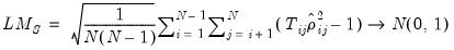
Pesaran CD
To address the size distortion of

and

, Pesaran (2004) proposes an alternative statistic based on the average of the pairwise correlation coefficients

:
 | (55.29) |
which is asymptotically standard normal for

and

in any order.
Further, Pesaran points out that for a wide array of panel data models, the mean of CD is exactly equal to zero for all

and all

, so that the CD test is likely to have good properties for both

and

small, and he provides Monte Carlo evidence to support this claim.
Baltagi, Feng, and Kao Bias-corrected Scaled LM
Baltagi, Feng, and Kao (2012) offer a simple asymptotic bias correction for the scaled LM test statistic:
 | (55.30) |
For a fixed effects homogeneous panel data model with

,

, and
, Baltagi,
et al. show that the scaled LM has an asymptotic bias term of
resulting from the incidental parameters problem since, for small

, the within residuals are estimated imprecisely. (Note that in
Equation (55.30) we extend the slightly Baltagi,
et al. scaled LM test to unbalanced designs by using the maximum of

for

and requiring that

as

).
Note that EViews will not compute the biased corrected LM statistic unless the equation was estimated with cross-section fixed effects.
Example
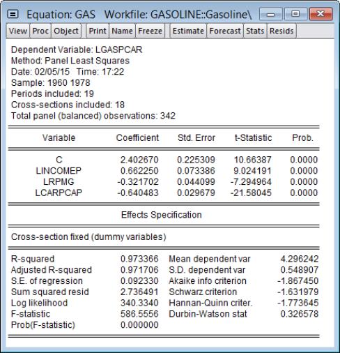
We illustrate the use of cross-section dependence tests for equation objects using an empirical example from Baltagi (2008) examining gasoline demand in 18 OECD countries over the period 1960–1978 (Table 2.8, p. 29).
We download the data and create a panel-structured workfile by entering the following command in the EViews command window
wfopen http://www.wiley.com///wileychi/baltagi/supp/Gasoline.dat lastobs=342
and clicking on in the import wizard to accept the default settings.
The equation of interest is a cross-section fixed effects regression of log motor gasoline consumption per auto (LNGASPCAR), on log real per capital income (LINCOMEP), log real motor gasoline price (LRPMG), log real motor gasoline price the log of the stock of cars per capita (LCARPCAP).
We estimate this fixed effect specification by entering the command:
equation gas.ls(cx=f) lgaspcar c lincomep lrpmg lcarpcap
which creates the equation object GAS and displays the estimation results:
Implicit in our approach to estimation in this example and in the validity of the computed t-statistics is the assumption that the errors for different cross-sectional units are uncorrelated.
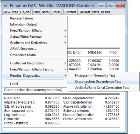
To test for the presence of cross-sectional dependence, we click on
EViews will compute the cross-section dependence tests and display the results in the object window:
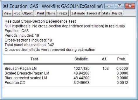
The top of the table displays the test hypothesis and information about the number of cross-section and period observations in the panel. The bottom portion of the table contains the test results.
The first line contains results for the Breusch-Pagan LM test. EViews shows the test statistic value, test degree-of-freedom, and the associated
p-value. In this case, the value of the test statistic, 1027.14 is well into the upper tail of a

, and we strongly reject the null of no correlation at conventional significance levels.
The next two lines present results for the two scaled Breusch-Pagan tests. Both the Pesaran scaled Breusch-Pagan LM, and the Baltagi
et al. bias-adjusted LM tests are asymptotically standard normal, and the test statistic results of 49.97 and 49.47 respectively, strongly reject the null at conventional levels. Note that in this example, the bias correction has a relatively small effect on the scaled LM statistic as

and

are of similar magnitude.
Since

is relatively small, we may instead wish to focus on the results for the asymptotically standard normal Pesaran CD test which are presented in the final line of the table. While the test statistic value of 3.25 is significantly below that of the scaled LM tests, the Pesaran CD test still rejects the null at conventional significance levels.
Arellano-Bond Serial Correlation Testing
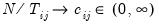
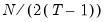
For models estimated by GMM, you may compute the first and second order serial correlation statistics proposed by Arellano and Bond (1991) as one method of testing for serial correlation. The test is actually two separate statistics, one for first order correlation and one for second. If the innovations are i.i.d. we expect the first order statistic to be significant (with a negative auto-correlation coefficient), and the second order statistic to be insignificant.
The statistics are calculated as:
 | (55.31) |
 | (55.32) |
 | (55.33) |
where

is the average
j-th order autocovariance.
(Note that this test is only available for equations estimated by GMM using first difference cross-section effects.)
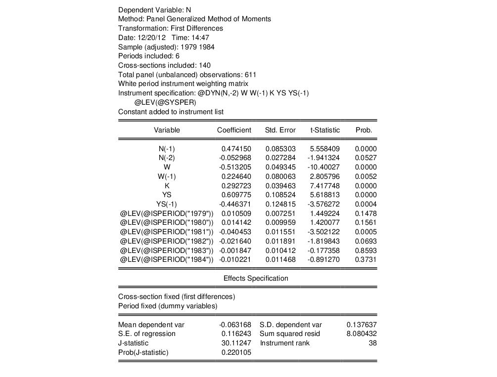
To perform the test click on . EViews will then calculate the test statistics for both first and second order correlation and display them in one table.
As an illustration, we again use the workfile ABOND_PAN.WF1 which contains data on a firm level panel, as examined in Arellano and Bond (1991), and Doornik, Bond and Arellano (2006). The following command estimates the GMM example used in the
“GMM Example” section, but uses ordinary standard error estimates, instead of the White period standard errors used above:
gmm(cx=fd, per=f, gmm=perwhite, iter=oneb, levelper) n n(-1) n(-2) w w(-1) k ys ys(-1) @ @dyn(n,-2) w w(-1) k ys ys(-1)
This equation replicates the estimates shown in Table 4(b), page 290, of Arellano Bond (1991).
Once estimated we click on to view the serial correlation test results. The table displays the results for a test of both first and second order serial correlation:
Although the original 1991 Arellano Bond paper does not display results for the first order test, the same data are used as an example in Doornik, Bond and Arellano 2006 (page 11), which does display corrected results for both tests.
The tests show that the first order statistic is statistically significant, whereas the second order statistic is not, which is what we would expect if the model error terms are serial uncorrelated in levels.
Pooled Mean Group Bounds Tests
The bounds test associated with univariate ARDL models (
“Bounds Test View”) may be computed for each cross-section in the panel.
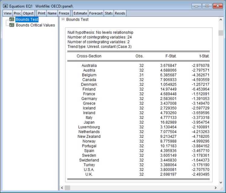
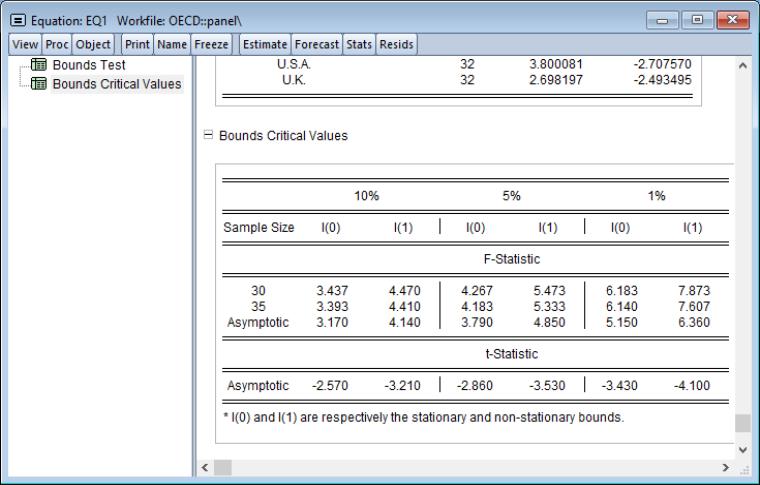
To perform these tests, click on . EViews will display a spool with the bounds statistics for each cross-section in the first node,
and with test critical values in the second node,
Pooled Mean Group Hausman (Similarity) Tests
The PMG estimator lies between mean group (MG) and pooled estimators which offer alternative assumptions about cross-sectional homogeneity.
At one extreme, the mean group estimator computes the average of coefficient estimates from separate cross-section specific equations. The estimation allows for complete heterogeneity of coefficients and variances, and ignores the fact that parameters may actually be identical across cross-sections.
At the other extreme are traditional pooled estimators such as the fixed and random effects estimators, which assume that the coefficients and variances are homogeneous across cross-sections (apart from limited exceptions such as individual effects).
The PMG allows intercepts, short-run coefficients and error variances to differ freely across groups, but constrains the long-run slope coefficients to be the same.
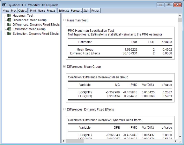
A useful diagnostic associated with these three estimators are Hausman-type (Hausman (1978)) tests applied to the difference between the MG and PMG estimators, and to the difference between PMG and dynamic estimators.
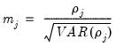
Formally, for long-run coefficient estimates

and

and corresponding covariances,

and

, under appropriate consistency and efficiency conditions, the test statistic,
 | (55.34) |
is distributed as a

, where

is the number of long-run parameters.
In the context of PMG estimation, one can construct two Hausman-type tests. The first considers the null of no difference in the consistent long-run coefficient estimates of the relative efficient PMG and the MG estimator. The second compares the PMG estimator to the relatively efficient pooled dynamic fixed effects estimator.
To compute the PMG Hausman tests, click on .
The output is a spool object displaying the Hausman test statistic value along with the associated p-value, along with additional output related to the difference of estimators, their variances, and the regression results from each of the mean-group and dynamic fixed effects regressions.
Pooled Mean Group Symmetry Tests
For PMG equations, the symmetry test associated with asymmetric NARDL regressors (
“Symmetry Test View”) can be derived for each cross-section. To compute the tests, click on . EViews will produce a spool with the NARDL symmetry test for each cross-section.
Pooled Mean Group Diagnostics
In addition to the specific tests outlined above, PMG estimation offers several diagnostic views.
Model Selection
The item on the menu allows you to view either a or a . The graph output shows the model selection value for the twenty “best” with the lowest criterion value. The table form of the view displays the log-likelihood value, AIC, BIC and HQ values of the best twenty models in tabular form.
Error-Correction Results
The error correction representation of the ARDL specification offers an easy-to-interpret representations of the cointegrating relationship between the dependent variable and the explanatory variables.
To see the individual cross-sectional short-run coefficients for the each of the cross-section EC equations, you can click on . The resulting display shows a spool containing each cross-section’s coefficients, standard errors, t-statistics and p-values.
See the discussion of the non-panel ARDL view
“Error Correction Output View” for additional background.Cointegrating Relation Graphs
To view the fitted cointegrating relation series for each cross section, you may click on the menu item .
See the discussion of the non-panel ARDL view
“Cointegrating Relation View” for additional background.