Views and Procedures
We turn now to a brief description of the views and procedures that are available for equations estimated using quantile regression. Most of the available views and procedures for the quantile regression equation are identical to those for an ordinary least squares regression, but a few require additional discussion.
Standard Views and Procedures
With the exception of the views listed under , the quantile regression views and procedures should be familiar from the discussion in ordinary least squares regression (see
“Working with Equations”).
A few of the familiar views and procedures do require a brief comment or two:
• Residuals are computed using the estimated parameters for the specified quantile:
. Standardized residuals are the ratios of the residuals to the degree-of-freedom corrected sample standard deviation of the residuals.
Note that an alternative approach to standardizing residuals that is not employed here would follow Koenker and Machado (1999) in estimating the scale parameter using the average value of the minimized objective function
. This latter estimator is used in forming quasi-likelihood ratio (QLR) tests (
“Quasi-Likelihood Ratio Tests”).
• Wald tests and confidence ellipses are constructed in the usual fashion using the possibly robust estimator for the coefficient covariance matrix specified during estimation.
• The omitted and redundant variables tests and the Ramsey RESET test all perform QLR tests of the specified restrictions (Koenker and Machado, 1999). These tests require the i.i.d. assumption for the sparsity estimator to be valid.
• Forecasts and models will be for the estimated conditional quantile specification, using the estimated

. We remind you that by default, EViews forecasts will insert the actual values for out-of-forecast-sample observations, which may not be the desired approach. You may switch the insertion off by unselecting the checkbox in the dialog.
Quantile Process Views
The view submenu lists three specialized views that rely on quantile process estimates. Before describing the three views, we note that since each requires estimation of quantile regression specifications for various

, they may be time-consuming, especially for specifications where the coefficient covariance is estimated via bootstrapping.
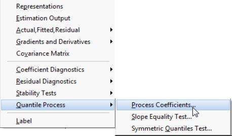
Process Coefficients
You may select to examine the process coefficients estimated at various quantiles.
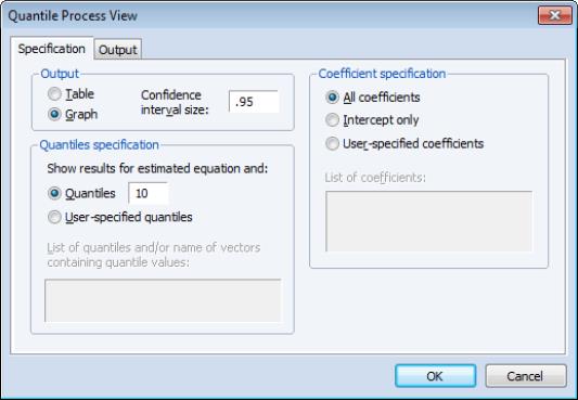
The section of the tab is used to control how the process results are displayed. By default, EViews displays the results as a table of coefficient estimates, standard errors, t-statistics, and p-values. You may instead click on the radio button and enter the size of the confidence interval in the edit field that appears. The default is to display a 95% confidence interval.
The section of the page determines the quantiles at which the process will be estimated. By default, EViews will estimate models for each of the deciles (10 quantiles,
). You may specify a different number of quantiles using the edit field, or you may select and then enter a list of quantiles or one or more vectors containing quantile values.
The radio buttons permit you to choose a subset of the coefficients to display. By default, EViews will produce results for all of the coefficients in your model. You may select to produce results only for the intercept, or you may select and enter a list of coefficient names to show results for specific coefficients. Entering, for example, “C(2) C(3)” will produce process results only for the second and third coefficients.
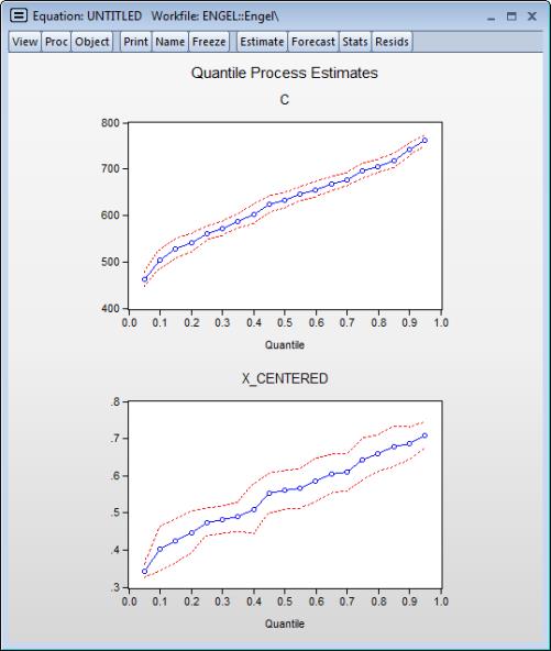
Here, we follow Koenker (2005), in displaying a process graph for a modified version of the earlier equation: a median regression using the Engel data, where we fit the Y data to the centered X series and a constant. We display the results for 20 quantiles, along with 90% confidence intervals.
In both cases, the coefficient estimates show a clear positive relationship between the quantile value and the estimated coefficients; the positive relationship for X_CENTERED is clear evidence that the conditional quantiles are not i.i.d. We test the strength of this relationship formally below.
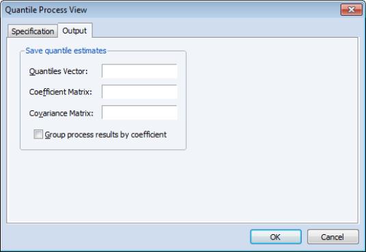
The page of the dialog allows you to save the results of the quantile process estimation. You may provide a name for the vector of quantiles, the matrix of process coefficients, and the covariance matrix of the coefficients. For the

sorted quantile estimates, each row of the

coefficient matrix contains estimates for a given quantile. The covariance matrix is the covariance of the vec of the coefficient matrix.
Slope Equality Test
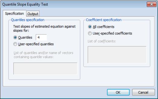
To perform the Koenker and Bassett (1982a) test for the equality of the slope coefficients across quantiles, select and fill out the dialog.
The dialog has two pages. The page is used to determine the quantiles at which the process will be compared. EViews will compare with slope (non-intercept) coefficients of the estimated tau, with the taus specified in the dialog. By default, the comparison taus will be the three quartile limits (
), but you may select and provide your own values.
In addition, you may use the section to specify a subset of coefficients to test. Simply click on the radio and enter a list of coefficient names to perform the tests on a specific set of coefficients. Entering, for example, “C(2) C(3)” will produce test equality only for the second and third coefficients.
The page allows you to save the results from the supplementary process estimation. As in
“Process Coefficients”, you may provide a name for the vector of quantiles, the matrix of process coefficients, and the covariance matrix of the coefficients.
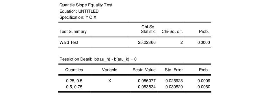
The results for the slope equality test for a median regression of our first equation relating food expenditure and household income in the Engel data set are provided below. We compare the slope coefficient for the median against those estimated at the upper and lower quartile.
The top portion of the output shows the equation specification, and the Wald test summary. Not surprisingly (given the graph of the coefficients above), we see that the

-statistic value of 25.22 is statistically significant at conventional test levels. We conclude that coefficients differ across quantile values and that the conditional quantiles are not identical.
Symmetric Quantiles Test
The symmetric quantiles test performs the Newey and Powell (1987) test of conditional symmetry. Conditional symmetry implies that the average value of two sets of coefficients for symmetric quantiles around the median will equal the value of the coefficients at the median:
 | (40.1) |
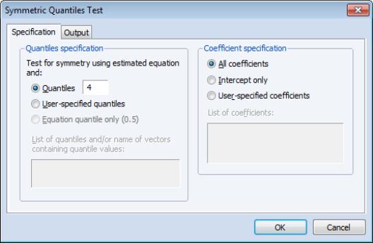
To perform the test, select and fill out the dialog.
By default, EViews will test for symmetry using the estimated quantile and the quartiles as specified in the dialog. Thus, if the estimated model fits the median, there will be a single set of restrictions:

. If the estimated model fits the

quantile, there will be an additional set of restrictions:

.
As with the other process routines, you may select and provide your own values. EViews will estimate a model for both the specified quantile,

, and its complement

, and will compare the results to the median estimates.
If your original model is for a quantile other than the median, you will be offered a third choice of performing the test using only the estimated quantile. For example, if the model is fit to the

quantile, an additional radio button will appear: . Choosing this form of the test, there will be a single set of restrictions:

.
Also, if it is known a priori that the errors are i.i.d., but possibly not symmetrically distributed, one can restrict the null to examine only the restriction associated with the intercept. To perform this restricted version of the test, simply click on in the portion of the page. Alternately, you may click on and enter a list of coefficient names (e.g. “C(3) C(4)”) to perform tests for specific coefficients.
Lastly, you may use the page to save the results from the supplementary process estimation. You may provide a name for the vector of quantiles, the matrix of process coefficients, and the covariance matrix of the coefficients.
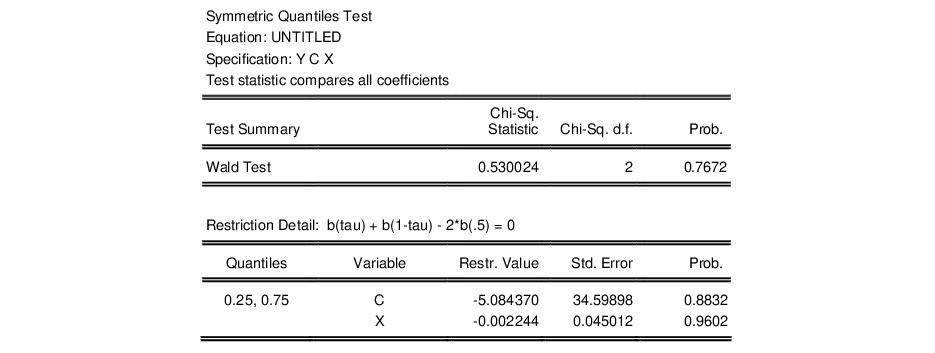
The default test of symmetry for the basic median Engel curve specification is given below:
We see that the test compares estimates at the first and third quartile with the median specification. While earlier we saw strong evidence that the slope coefficients are not constant across quantiles, we now see that there is little evidence of departures from symmetry. The overall p-value for the test is around 0.75, and the individual coefficient restriction test values show even less evidence of asymmetry.