Automatic ARIMA Forecasting
Automatic ARIMA forecasting is a method of forecasting values for a single series based upon an ARIMA model.
Although EViews provides sophisticated tools for estimating and working with ARIMA models using the familiar equation object, there is considerable value in a quick-and-easy tool for performing this type of forecasting. EViews offers an automatic ARIMA forecasting series procedure that allows the user to quickly determine an appropriate ARIMAX specification and use it to forecast the series into the future.
Methodological Background
The series

follows an ARIMAX(

) model if:
 | (11.47) |
(for notational simplicity, we ignore here the possibility of seasonal ARMA terms).
Often the exogenous variables

are simply a single constant or trend term. In such cases the only decision the forecaster has to make to set up his forecasts, is the form of the dependent variable, the level of differencing, and the number of AR and MA terms (
i.e. – choose

and

). One method of choosing the number of AR and MA terms is through model selection/evaluation techniques.
ARIMAX models may be estimated through a number of different methods, including transforming the model into a non-linear least squares specification, or using GLS or maximum likelihood estimation. Since maximum likelihood estimation does not require dropping observations from the start of the sample, or backcasting to create observations, it lends itself nicely to model selection/comparison algorithms.
Automatic Model Specification
Specifying the ARIMAX model used for forecasting can be split into four steps:
1. Selecting any transformations of the dependent variable, such as taking logs.
2. Selecting the level of differencing of the dependent variable.
3. Selecting the exogenous regressors.
4. Selecting the order of the ARMA terms.
EViews’ automatic forecasting procedure automatically performs steps 1., 2. and 4. The procedure will not select a set of exogenous regressors automatically, although it does allow the user to specify which regressors to include. As such we refer to the procedure as performing “automatic ARIMA forecasting”, rather than “automatic ARIMAX forecasting”.
Transformations and Differencing
Selecting a dependent variable transformation is often based on an underlying economic theory. Common transformations are to take logs, or to use the Box-Cox transformation. However it may be possible to determine whether taking logs is appropriate through a rule-of-thumb method which runs two simple regressions:
• 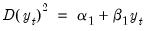
• 
A comparison is then made between the
t-statistic on

and that on

. If the t-statistic on

is lower than that on

, the log model is preferred.
The logic behind this test is that taking natural logs is often used on variables with an exponential growth rate — the change in growth increases or decreases over time. Such data, when used in a least squares estimation involving differences, will suffer from heteroskedasticity (since the change, or difference, in the data is not constant). Taking logs linearizes the relationship, and alleviates the problem of heteroskedasticity. Each of the two regressions is a simple, crude, test for heteroskedasticity, with a low
t-statistic on

suggesting homoskedasticity rather than heteroskedasticity. Regression 1 being “more homoskedastic” than regression 2 would suggest the data does not need to be logged. Conversely, regression 2 being “more homoskedastic” than regression 1 suggests the data should be logged.
Step 2 is to decide upon appropriate level of differencing for the (possibly transformed) dependent variable. Following the suggestion of Hyndman and Khandakar (HK, 2008), EViews uses successive unit root tests to determine the correct level of differencing. HK recommend preferring under-differencing the model as opposed to over-differencing when forecasting (themselves following the earlier work of Smith and Yadav 1994). Consequently HK suggest using a unit-root test with the null-hypothesis of no unit-root, such as the KPSS test.
The KPSS test is first run on the data with no differencing. If the test rejects the null hypothesis, the data is then differenced and the test run again. This continues until we can no longer reject the null hypothesis.
ARMA Selection
EViews uses model selection to determine the appropriate ARMA order. Model selection is a way of determining which type of model best fits a set of data, and is often used to choose the best model from which to forecast that data.
Information Criteria
Information criteria are the most common model selection tool used in econometrics. EViews supports three types of information criteria for most estimation methods; Akaike Information Criterion (AIC), Schwarz Criterion (SIC or BIC), and the Hannan-Quinn Criterion (HQ). Each of these criteria are based upon the estimated log-likelihood of the model, the number of parameters in the model and the number of observations. Additional detail may be found in
Appendix E. “Information Criteria” .
One issue with using information criteria is that the models not only need to be estimated on the same set of observations across models, but the dependent variable must also be of the same scale. You cannot, generally, evaluate models across transformations and differences of the dependent variable.
Thus information criteria based model selection can only be used in ARIMA models to determine the number of ARMA terms. It cannot be used to determine any transformations or differencing of the dependent variable. Determining the number of ARMA terms is typically done by specifying a maximum number of AR or MA coefficients, then estimating every model up to those maxima, and then evaluating each model using its information criterion.
Estimation of ARIMAX models by maximum likelihood makes comparison of different models using information criteria simple, since the log-likelihood is estimated as part of the estimation procedure. Once each model is estimated, its criterion can be calculated, and then the model with the lowest criterion value is chosen.
Mean Square Error (MSE) Evaluation
A second method of model selection is that of in-sample forecast evaluation. Here each model is estimated on a sub-sample of data (usually the first 80%-90%), and then forecasted over the remaining data (the remaining 10%-20%). Since we have data for the actual values of the dependent variable over the sub-sample forecast period, we can compare the forecasts with the actual data and calculate the mean square error (MSE):
 | (11.48) |
where

is the number of periods in the forecast subsample, and

is the number of periods in the full sample.
Each model is estimated and forecasted over the smaller sample, and the model with the smallest MSE is chosen.
Starting Values
Maximum likelihood estimation of ARMA models requires starting values for the coefficients. EViews' automatic ARMA estimation routine uses a data-based algorithm to determine starting values. However if estimation using these starting values fails to converge, EViews will then try a set of fixed starting values. If that estimation too fails to converge, EViews will finally try a set of random starting values.
Forecasting
Once the best model's transformation, differencing and ARMA length has been selected, either through information criteria or via MSE, the model is used to calculate the final forecast.
Forecast Averaging
An alternative approach to selecting the “best” ARIMA model and then forecasting from it is to forecast from each of the individual ARIMA specifications under consideration, and then average over those forecasts to produce a final forecast.
EViews allows to forms of forecast averaging when performing automatic ARIMA forecasting; Smoothed Akaike Information Criterion (SAIC), and Bayesian Model Averaging (BMA). For details on these forecast averaging methods, see
“Forecast Averaging”.
Since both of these methods are based upon information criteria, the same restrictions apply to them as to using information criteria for model selection—namely the samples used for estimation must be the same, and the dependent variable (the variable to be forecasted) must have the same scale. Consequently, when performing forecast averaging on ARIMAX models, only the subset of forecasts from models with the same transformation and differencing can be averaged.
When performing forecast averaging under automatic ARIMA forecasting, EViews then selects the form of transformation and differencing using the methods outlined above, and then forecasts from each combination of ARMA order to produce the set of forecasts available for averaging. The final produced forecast is then the weighted average of those forecasts.
Performing Automatic ARIMA Forecasting in EViews
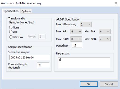
To forecast a series automatically using ARIMA models, open up the series and click on which will bring up the Automatic ARIMA Forecasting dialog:
The first section of the Specification tab of the dialog allows selection of the type of dependent variable transformation by using the Transformation radio buttons. The default selection, Auto (None/Log), instructs EViews to perform the rule-of-thumb test outlined above to determine whether to log the dependent variable or not. The remaining choices perform no transformation, take logs, or use the Box-Cox transformation. If Box-Cox is selected, a power parameter for the transform must also be provided. Auto and Log should only be used if your data are strictly positive.
The ARIMA Specification area of the dialog selects the type of ARIMA models that will be used during model selection or forecast averaging. To select the maximum level of differencing to be tested use the Max differencing dropdown box. EViews will perform successive KPSS tests on different levels of differencing, starting from zero and stopping only when the null hypothesis of the KPSS test cannot be rejected, or the maximum level of differencing selected by the user is reached.
The Max. AR, Max. MA, Max. SAR and Max. SMA dropdowns select the maximum order of the AR, MA, SAR and SMA terms of the ARIMA model. The periodicity of the seasonal terms can be entered in the Periodicity box. If the workfile is dated, EViews will default the periodicity to the number of observations per year, but this may be overwritten to model non-annual seasonalities.
The Regressors box allows entry of any exogenous regressors in the model. By default a constant is included.
The final section of this tab of the dialog includes the Estimation Sample box and the Forecast length box. Estimation Sample determines the observations used in determining the appropriate ARIMA model to use for forecasting - it specifies the observations used for the rule-of-thumb regressions determining whether to log the dependent variable or not, the observations used in the successive KPSS tests for determining differencing order, as well as the observations used in the estimation of the individual ARMA models.
Forecast length specifies h, the number of observations that will be forecasted after estimation. The forecast sample will start immediately after the last observation of the estimation sample and will continue for h observations. Note the workfile must be sized such that h observations exist in the workfile after the estimation sample.
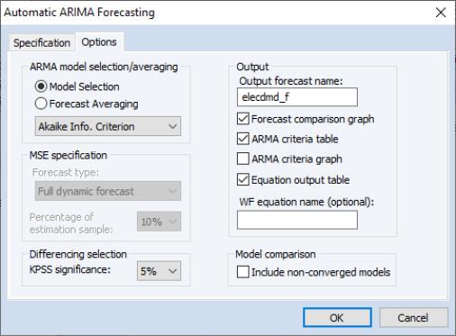
The Options tab of the dialog provides further options on model selection and output:
The ARMA model selection/averaging box selects the method used to choose the appropriate ARMA model, or the method of forecast averaging. The Model Selection and Forecast Averaging radio button select whether to use model selection or forecast averaging, with the dropdown box below them allowing selection of which type of model selection (AIC, BIC, HQ or MSE based), or forecast averaging (SAIC or BMA) to use.
If MSE based model selection is used, the MSE specification area allows specification of the MSE calculations. Forecast type selects whether the in-sample forecast used to compute the MSE is a dynamic forecast or a static forecast. The Percentage of estimation sample dropdown selects the part of the estimation sample (chosen on the Specification tab) that is used for in-sample forecasting for calculating the MSE.
The KPSS significance dropdown specifies the significance level to use when determining whether the null hypothesis of the KPSS test is rejected or not during differencing selection.
The Convergence control section includes a checkbox for specifying whether to include non-converged models amongst those included in model selection or forecast averaging. If left unchecked, only ARMA estimations that EViews believes are fully converged will be included in the selection/averaging. If the output of the automatic ARIMA forecasting procedure indicates that a large number of models didn’t converge, and it is believed this may be due to border solutions or a very flat likelihood, checking this option may improve the accuracy of the final forecast.
The Output area allows customization of the output from the procedure. The Output forecast name: box is used to name the final forecast series in the workfile. By default it is filled in with the name of the underlying series followed by an “_F”.
Checking the Forecast comparison graph check box will produce a graph containing the final forecast (either the forecast from the selected model, or the averaged forecast) along side the forecasts from every other ARMA model considered. The final forecast will be colored red, with the other forecasts in grey. Note, the graph is only displayed if the Forecast length specified on the Specification tab is greater than zero (i.e.—a forecast is actually performed).
The ARMA criteria table and ARMA criteria graph check boxes specify whether to include a table, or graph, of the “best” 20 models used during model selection or forecast averaging. The graph shows the model selection value for the twenty “best” models. If you use either the Akaike Information Criterion (AIC), the Schwarz Criterion (BIC), or the Hannan-Quinn (HQ) criterion, the graph will show the twenty models with the lowest criterion value. The table form of the view shows the log-likelihood value, the AIC, BIC and HQ values of the top twenty models in tabular form.
Finally, If Model Selection is chosen, selecting the Equation output table option produces a standard EViews ARMA equation output table of the final selected equation. Similarly, entering a name in the WF equation name (optional) box will create a new equation object in the workfile with the same specification as the final chosen model. Outputting an equation object allows performance of post-estimation diagnostics and tests.
Example
As an example of using automatic ARIMA forecasting in EViews, we forecast monthly electricity demand in England and Wales, using the workfile “elecdmd.wf1”. This workfile contains monthly electricity demand data from April 2005 until April 2014 (in the series ELECDMD), as well as real GDP data for the UK (a good proxy for real GDP in England and Wales) and average monthly temperature (series TEMPF).
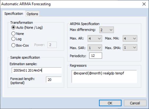
We will use automatic forecasting to forecast the ELECDMD series from May 2014 until December 2015. To do this we open up the series and click on , which brings up the automatic ARIMA dialog:
We'll let EViews decide on the best transformation by selecting in the Transformation box.
We select an estimation sample of January 2005 until April 2014. In the ARIMA Specification area we'll leave most of the settings at their default values, other than, since our data has clear seasonal patterns, changing the maximum number of seasonal terms from 0 to 1.
We also add some monthly dummy variables using the @expand(@month) keyword, and add REALGDP and TEMPF as exogenous regressors.
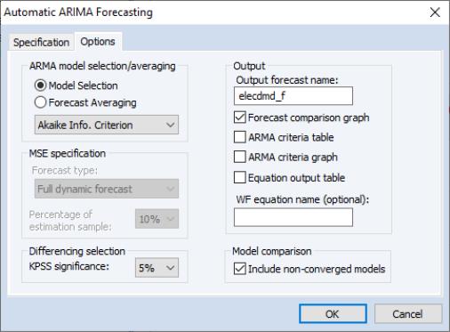
On the Options tab, we keep most of the settings at their default values.
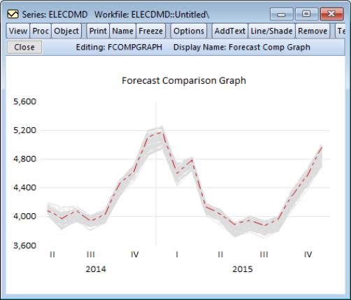
So that we may compare the forecasts of the ARIMA models, we select the Forecast comparison graph checkbox.
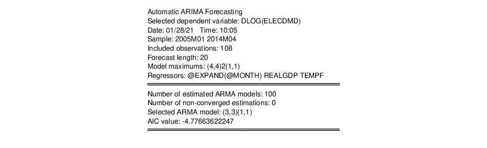
The results of the auto-ARIMA estimation are shown below:
The summary table indicates that out of the 100 different models estimated, the chosen ARMA was a (3,3)(1,1) model. The automatic transformation detection decided that logging and first-differencing our underlying series, ELECDMD, would provide a better model.
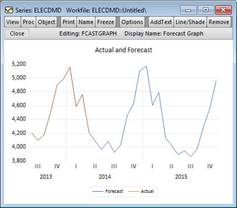
The indicates that the chosen model forecasted the actual values pretty well.
The shows that each of the 100 models picked up the same cyclical patterns pretty well (undoubtedly due to the inclusion of our exogenous regressors).