Graphs and Tables
Graph Line and Shade Transparency
EViews 13 now allows you to customize the opacity (transparency) levels of individual lines and shades in a graph. By exercising fine control over the visibility of stacked graph elements, you can uncover previously hidden features of your data.
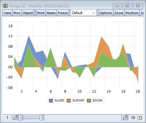
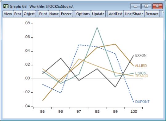
When plotting multiple data for series in prior versions of EViews, the graph for data from one series could obscure the data of another. For example, the following area graph shows time series graphs for three series in a group object (ALLIED, DUPONT, and EXXON):
In this graph, data for ALLIED is drawn first, followed by the data for DUPONT, and then by the data for EXXON. Notice that the areas for the later drawn series obscuring the areas for the earlier. Note in particular, that the values of EXXON for observations hide the corresponding values of DUPONT and ALLIED, particularly for observations from 9 to 16.
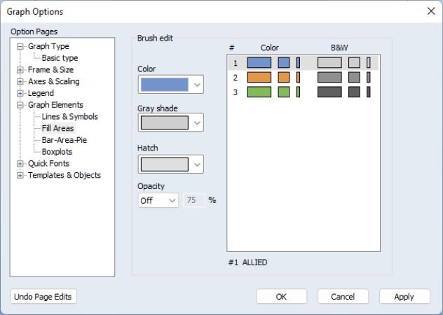
EViews 13 allows you to adjust the opacity of individual graph elements to improve the visibility of others. To set the opacity for one or more elements, double click on the graph to display the graph options, or select on the Options button on the button bar, then select the node.
Opacity levels may be set for individual Lines and Fill Areas by clicking on an entry in the right hand side of the graph to select a graph element and then entering a number from 0 to 100 in the Opacity % edit field:
You may set levels for more than one element simultaneously by SHIFT or CTRL clicking to select multiple elements, and then applying the desired setting.
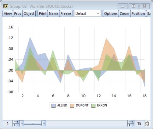
Here is the same graph after setting the of all three of the fill elements to “50”:
Note the additional visible detail in the values of the ALLIED and DUPONT series for observations 9 to 16. In particular, the values of ALLIED, the first drawn series were virtually invisible in the earlier graph, but now show an obvious sawtooth pattern.
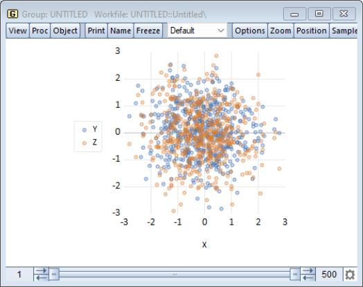
Similarly, turning down the opacity in a dense scatterplot can show additional detail:
Judicious use of transparency settings makes possible the production of graphs that show data in ways that were not previously possible.
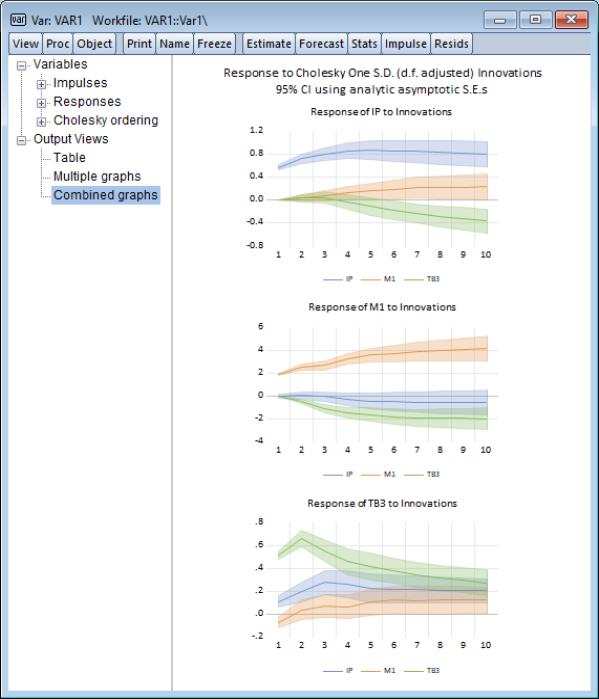
The new multiple shaded confidence intervals in combined impulse-response graphs (
“Enhanced Impulse Response Display”) employ this feature and hint at the types of graphs that may be produced:
To set opacity levels by command use the
Graph::setelem command to select an element and add the
lineopacity (for lines) and
fillopacity (for fills) keywords to set the desired opacity values.
Setting the level to 0.0 (0%) will make the object completely transparent while 1.0 (100%) will make the object completely opaque.
For example,
gr1.setelem(2) lineopacity(.5)
In our example, the second line in the graph was set to be 0.5 (50%) opaque.
Custom Graph Data Labels
Providing labels for data values can be an important tool for enhancing the information content of graphical presentation of data. EViews 13 offers new automatic tools which make it easy to augment your graphs with informative custom data and observation-based labels.
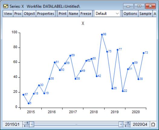
Recall that in EViews 12 and earlier, EViews offered option to use data values to label each of the observations in a graph.
While often quite useful, this option had limitation. For one, labeling observations with data values was an all or nothing proposition; data values were either displayed for all observations or for none of the observations. Further, customization of the format of the data labels was limited to specifying a size and font of the data label, and showing or not showing an open or closed circle symbol alongside the label.
EViews 13 enhances the ability to label observations to provide you with greater control over your data labeling. You may now:
• Label all observations, no observations, the first observation, or the last observation.
• Specify the content of the data label by using the data value, the observation, the name of the series, or arbitrary text.
• Modify the font, font size and position of the data label.
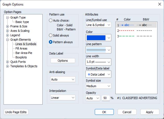
Data labeling is controlled in thedialog. Click on the button or double-click on the graph to display the dialog then select and and select one or more the elements on the right-hand side of the dialog The Data label settings will be displayed when you choose or to display. To show data labels, select one of the three entries in the drop-down control (open circle and data label, closed circle and data label, data label):
Here, we have selected the with a closed circle symbol.
By default, when you choose a data label setting, EViews will display labels for all observations.
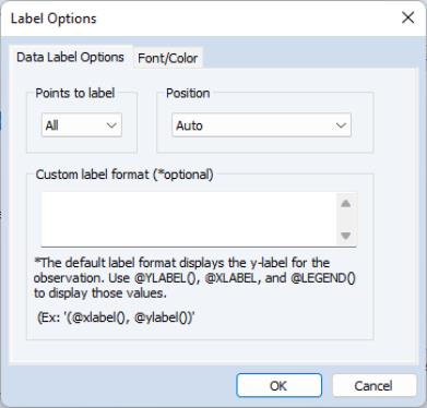
EViews 13 introduces the ability to customize the data label display. Click on the large button under the entry in the middle of the dialog to display the dialog:
The first tab provides basic labeling options:
• The radio buttons in the bottom left allow you to choose between displaying labels for All, the First, or the Last observation.
• The Position drop down lets you choose to display the label using Auto positioning, or to the Right of observation, Left of observation, Above observation, Below observation, or Center on observation.
• The Label Format edit field allows you to specify the content of the label. You should enter text for the specification in the edit field. The special functions @xlabel() and @ylabel() instruct EViews to use the corresponding X-values and Y-values of the observations as the label; the function @legend() corresponds to the legend value for the data element. All other text will be used in the label as given. You may use the ENTER key format the label in multiple lines.
The second tab of the dialog specifies font family, size, and color settings, as well as special text effects like underlining and strikethrough.
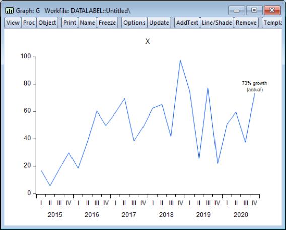
Below, we use the Last observation setting to label the last data point using the Y-value to form a custom data string “% growth (actual)”, by entering
@ylabel()% growth
(actual)
in the edit field. Note that the carriage return in the edit field is used to create a multi-line label.
Importantly, if an observation were to be added to end of the graph, the data label would automatic change to reflect the new value as well as move to proper location above new observation.
Similarly, you may use custom data labels in place of a legend. In this example, the legend was disabled and we activate the custom data label for the last observation, using a
@legend()
specification in the edit field.
Note that a custom data label differs from a custom text label. Data labels are attached to an observation in the graph, while custom text labels may be placed anywhere in the graph. While custom text labels may be placed so that they appear related to specific data values, it takes a bit of work to tie them to the observation data values. In contrast, a custom data label is designed to be linked to the observations so it may easy to attach label text to the first, last, or all of the observations.
Customizable Geomap Labels
In EViews 13, you may now use more than one attribute, along with custom text and formatting, to label the shapes in your geomap.
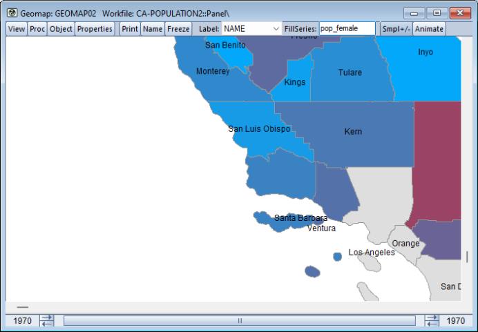
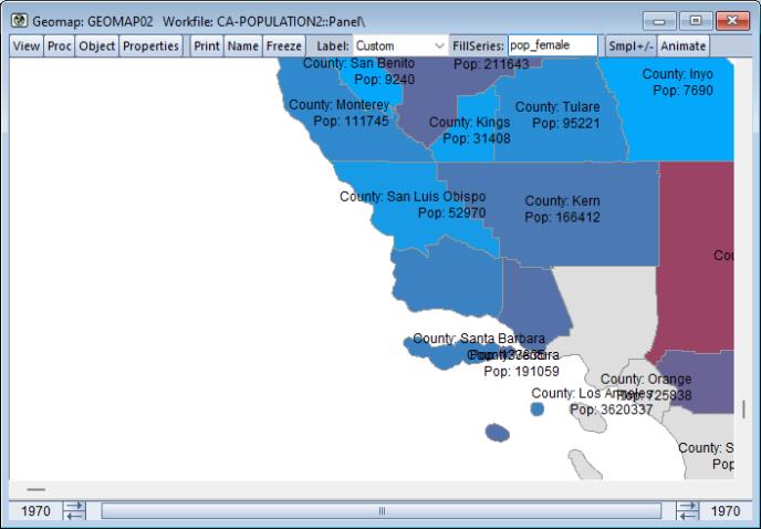
Note that the ability to attach labels to the shapes in a geomap is one of the most important tools for customizing the display of area data. In the simplest example, we may display the name of a geographic region in each area of a geomap display. For example, we may display the county names in our geomap display of the county areas in the State of California, USA.
Here, the county names are one of several attributes of the geomap shapefile data, which pairs each shape are with one or more pieces information. Each shape in the file might have information on “Name”, “Population”, “Income”, “Population % change”, etc.
In EViews 12, you could display a geomap with a single label taken from a single attribute, as in the example above. So while you could instruct EViews to use the “Name” attribute to display county name, or the “Population” attribute to show population, you could not display labels showing both county name and population in each shape.
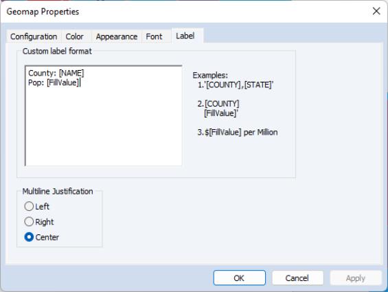
EViews 13 removes this single attribute restriction, allowing you to use multiple attributes to construct an area label. Furthermore, you may add custom text to your label, and apply custom formatting including, font family and size, and multi-line display.
Here we use the attribute “NAME” and the value of the workfile series POP_FEMALE to create a custom, multi-line label for each shape:
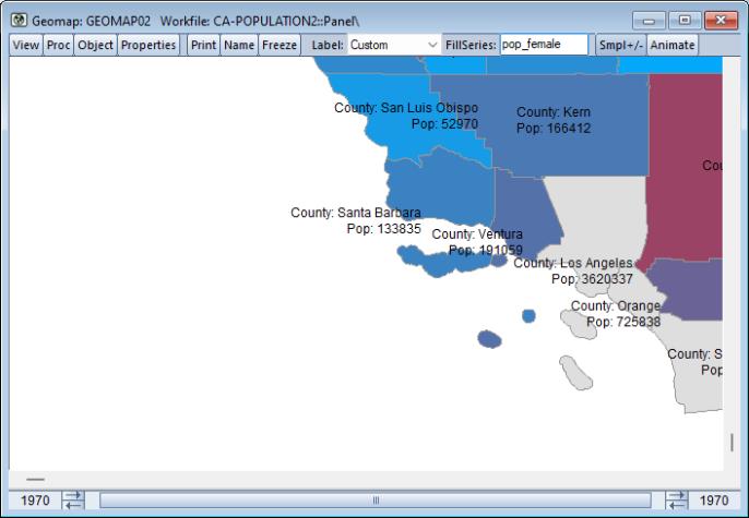
Should the default position of a label not be ideal, it may be adjusted manually. Simply click and drag a label to its desired location:
Note the improved labeling of the offshore areas in Santa Barbara, Ventura, and Los Angeles counties.
For command support, see:
•
Geomap::setjust to set the display justification for multi-line area labels.
•
Geomap::setshapelabel to used attribute or value labels, or to create a custom label to use when labeling shapes.
High-Low-Median Colormap Preset
EViews supports colormaps where you can define sets of rules that translate numeric values into colors. These colormaps may then be used when setting the text or fill color for series or group spreadsheets, or the fill colors in geomaps.
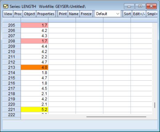
EViews 12 offers a number of predefined colormaps for common settings, such as the colormap which negative values will be displayed as red and positive values will be displayed as black. In addition to EViews 12 pre-specified presets, EViews 13 includes a new preset which allows users to identify the high, low, and median observations.
To apply this preset to a displayed series spreadsheet, click on then select the or as desired:
Choose in the dropdown, and choose the colors appropriately. Click on to display the spreadsheet with the colormap applied:
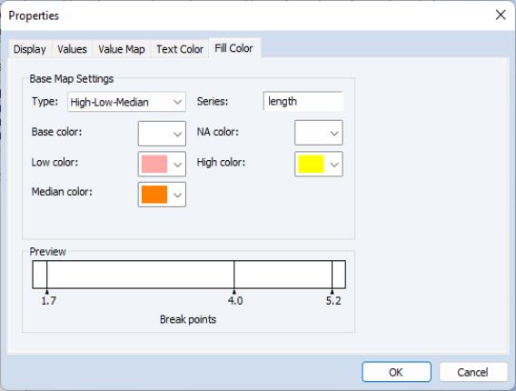
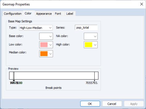
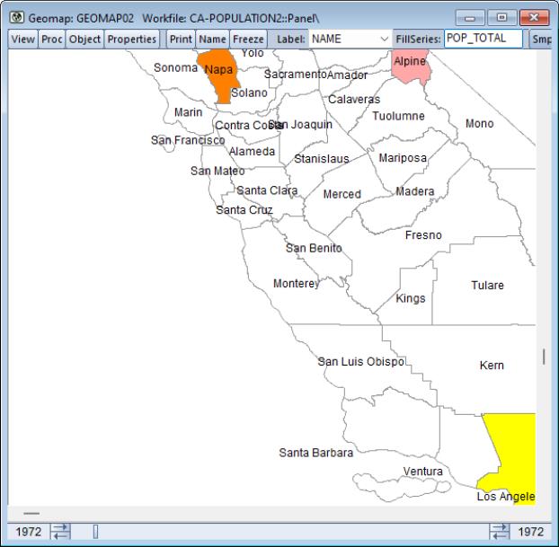
For geomaps you will click on , then select the tab and choose in the dropdown,
Click on to display the geomap with the colormap applied:
Applying a high-low-median colormap is done using the existing setfillcolor proc and the “t=hilo” option:
geomap01.setfillcolor(t=hilo) mapser(POP_TOTAL) min(-352258.35) max(7408557.35) highclr(@RGB(255,168,168)) lowclr(@RGB(255,255,128)) medianclr(@RGB(255,190,96))
Table Search
EViews 13 introduces the ability to search cells within a table, both interactively and in programs.
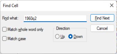
To locate a particular value or string in a table interactively, first ensure that the table window is active, then press Ctrl+F or select from the main menu to display the dialog.
When searching, you have the option to match the whole word, match case, and the specify the search direction. After making any selections, press the button to locate a matching cell.
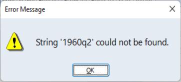
If no match is found, EViews will produce an error message,
If a match is found, the first located corresponding cell within the table will be selected:
Subsequent searches will select the next matching cell. If the end of the table is reached, EViews will resume the search from the beginning or end of the table, depending on the search direction.
Perhaps more importantly, EViews 13 provides a new table data member @find, that provides a string containing cell identifiers which satisfy a boolean condition. The condition may be expressed as a mathematical (using numerically interpreted values of the cell contents) or string comparisons, using cell references.
The table data member,
@find("expression")
where expression can be a mathematical or string expression, returns a string containing the cell identifiers which meet the bool expression.
For example,
string s = tab1.@find("[b1:c15]>0.3")
returns the list of cells between cell B1 and C15 which have a value greater than 0.3.
string s = tab1.@find("[a1:e67]== ""1949q4""")
returns the list of cells between A1 and E67 which match the string “1949q4”, ignoring case (note: string comparisons in @find ignore case).
string s = tab1.@find("[@all]==0.5")
returns the list of cells in the table that are equal to 0.5.
string s = tab1.@find("@instr([@all],""in"")")
returns the list of cells in the table that contain the substring ‘in’.
string s = tab1.@find("[b3:c5]<[d5]")
returns the list of cells between B3 and C5 that have a value less than the value of cell D5
string s = tab1.@find("@left([@all], 2)==""cp""")
returns list of cells in the table that start with the string “cp”.
Conditional Table Cells
Many EViews table customization procedures allow you to specify ranges of cells. For example,
Table::setfillcolor allows you to specify the background color for the specified cells.
There are cases when you may wish to perform operations on cells in a table, but only under certain conditions. Suppose, for example, that you have a table with annual data on each row and you want to identify each row where there is a decrease in value in column 3 when compared to the value for the previous row (year). The goal is to apply custom text or cell formatting to these rows.
Fortunately, EViews allows you to identify the desired cells using a conditional target range specification comprised of a target_range and a boolean_expression. You may specify the conditional target cells using the syntax:
target_range if boolean_expression
where target_range gives the range of potential cells of interest, “if” is a keyword, and boolean_expression provides indicators for which of the target_range cells to use.
For example, the command
tab1.setfillcolor(A2:A7 if [A2:A7]<[A1:A6]) red
will only set the fill color to red for the target cell range, if the decreasing value condition holds.
Similarly, the table @find data member allows you to obtain a string list containing the cells in a table range that satisfy a condition. The syntax for @find requires a find_expression:
table_name.@find(find_expression)
where find_expression simultaneously specifies the range of cells to consider and the boolean expression for whether each cell should be used.
For example the command
string s = tab1.@find("[b1:c15]>0.3")
returns the list of cells between cell B1 and C15 which have a value greater than 0.3.
string s = tab1.@find("@instr([@all],""in"")")
returns the list of cells in the table that contain the substring ‘in’.
string s = tab1.@find("[b3:c5]<[d5]")
returns the list of cells between B3 and C5 that have a value less than the value of cell D5
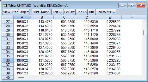
Fixing Rows and Columns in Tables
EViews 13 now allows you to fix rows and columns in the display of a table so that these rows and columns are always in view as you scroll the remaining cells of the table.
There are times when it is useful to lock one or more rows or columns in a table so that those rows and columns are always in view. Depending on the contents of the table, the first few rows or columns in your table may contain identifying information about the data cells within the table. When searching for a specific cell or set of cells, fixing the display of these identifiers makes this task much easier. This is especially useful for tables containing a large number of columns or rows.
This situation often occurs, for example, when working with tables where the first row contains column names and the first column contains observation IDs. In the case when the table is scrolled both vertically and horizontally such that the 20th column and the 100th row of a table is in view it may be helpful to see the column names and observation IDs to have provide context to the contents of the cell.
Fixing columns and rows in a table can be done by pressing the button in a table object button bar. Then,
• To fix only the first row, select . If more than 1 row is to be fixed, select a cell in the first row after the last desired fixed row and then from the menu select . For example, to fix the first 3 rows of table, select a cell in the fourth row and then select .
• The process for fixing columns is the same as fixing rows with the obvious exception of selecting
• Similarly, after navigating through the proc menu, the columns proceeding the current selected cell will be fixed. Note the fixed columns and rows will be denoted in the table by a black cell border.
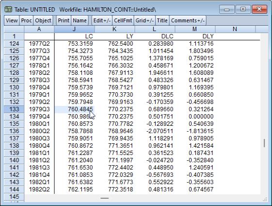
In the image below which fixes the first row and column of the table, you can see the date column (column A) and the series names (row 1) are in view despite the table being scrolled vertically 123 rows and 13 columns where row 124 is the first row, and column J is the first column displayed.
The fixed columns are denoted by a black cell border that extends from the top to bottom of the table and the fixed rows are separated by a similar black border that extends from the left to right of the table.
With fixed headers and rows, we can readily identify the selected cell as being the value for LC for 1979q3.
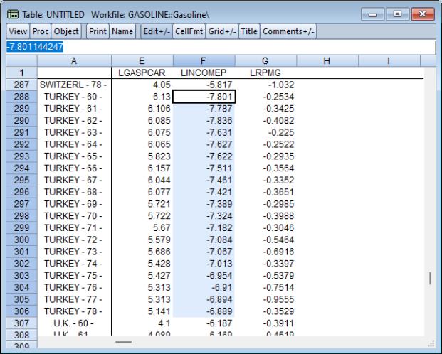
In this second example, the fixed first row and column of the table makes it easy to identify the LINCOMEP values for Turkey from 1960 to 1978 despite the fact that the displayed values are for the 288th row and column F of the table.
To unfix any fixed rows or columns, simply press the button and either select or . Note: the cell selection is ignored when unfixing rows or columns.
Note that fixed rows and columns are saved with the table when the workfile is saved to disk.
See
Table::fixcol,
Table::fixrow, and
Table::fixrowcol.Fixing the beginning set of columns in table is accomplished via the table name followed by the
fixcol proc and the number of columns to be fixed. This procedure force the number of specified columns to always be in view regardless of the horizontal scroll position. Once fixed, a black cell border will separate the fixed and unfixed rows and columns.
Similarly, to fix the beginning set of rows in the table use the fixrow keyword followed by the number of rows to be fixed.
For example, the commands
tab1.fixcol 2
tab1.fixrow 1
will fix the first two columns and the first row of the table.
Alternately you may fix both the row and column using the single command
tab1.fixrowcol 1 2
You may clear the fixed rows and columns using
tab1.fixcol 0
tab1.fixrow 0
or
tab1.fixrowcol 0 0