Econometrics and Statistics
EViews 13 offers a exciting new additions and improvements to its set of econometric and statistical features. The following is a brief outline of the most important new features, followed by additional discussion and pointers to full documentation.
ARDL Estimation
EViews 13 offers improvements to existing tools for analyzing data using Autoregressive Distributed Lag Models (ARDL), featuring estimation of Nonlinear ARDL (NARDL) models which allow for more complex dynamics, with explanatory variables having differing effects for positive and negative deviations from base values.
The classical ARDL framework assumes that the long-run cointegrating relationship is a symmetric linear combination of regressors. While this is a natural starting assumption, it does not match the behavioral finance and economics literature approach to modeling nonlinearity and asymmetry (Kahneman, Tversky, and Shiller, 1979). In response, Shin (2014) proposes a nonlinear ARDL (NARDL) framework in which short-run and long-run nonlinearities are modeled as positive and negative partial sum decompositions of the explanatory variables.
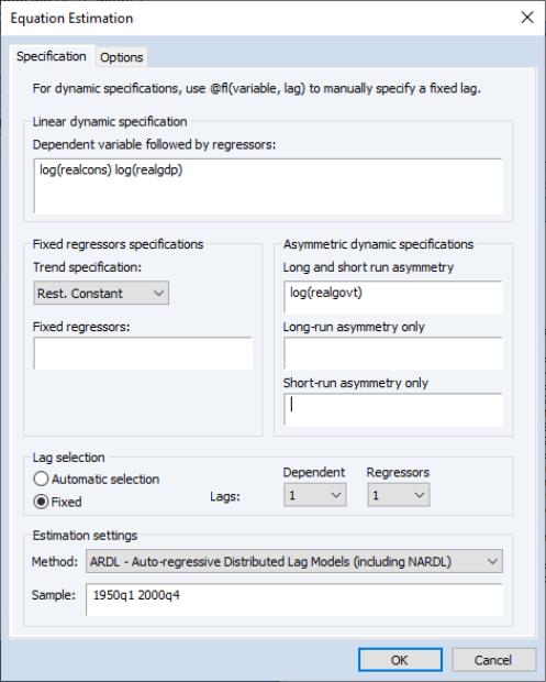
From the main EViews menu, click on or type the command equation in the command line to open the equation dialog. Then select the from the dropdown to display the ARDL dialog:
In the , you should a enter a list of variables consisting of the dependent variable followed by any symmetric ARDL distributed lag regressors. At a minimum, the edit field must contain the dependent variable.
Exogenous regressors, including deterministics, may be specified in the section. Trend regressors corresponding to the five deterministic cases discussed (, , , , ) may be specified using the dropdown. All other exogenous regressors (those apart from the constant and the trend) should be specified in the edit field.
Asymmetric distributed lag regressors may be listed under . In particular, the edit field may be used to specify regressors which are asymmetric in both the long-run and short-run. Regressors which are asymmetric only in the long-run may be specified in the edit field, while those which are asymmetric exclusively in the short-run are specified in the edit field.
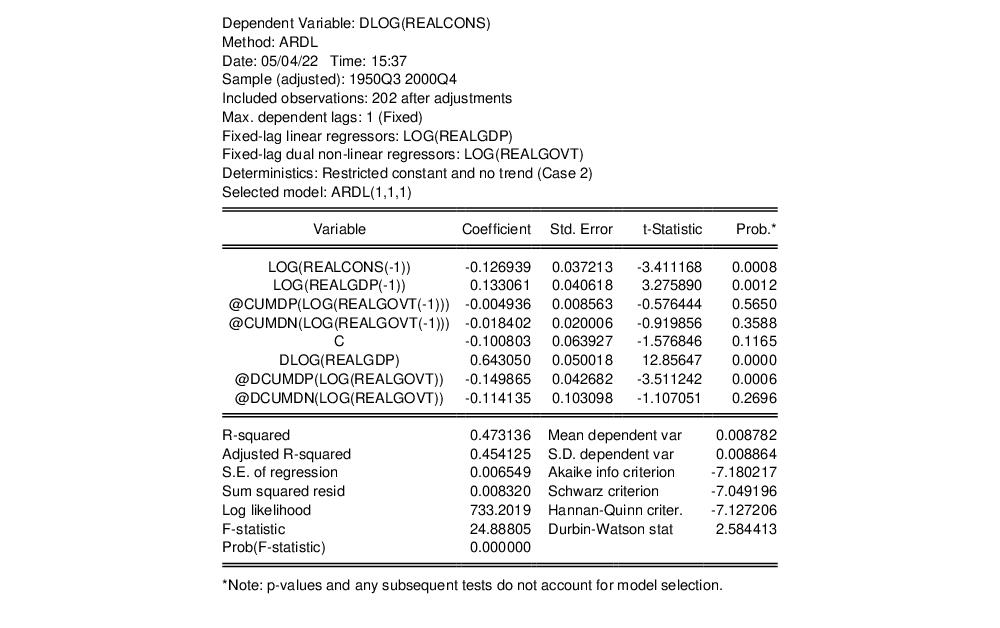
In addition to the support for estimating nonlinear ARDL specifications, EViews 13 offers a number of new ARDL diagnostics. These diagnostics are designed to help you examine the dynamic behavior of your variables, the long-run properties of your specification, and the appropriateness of your model.
Pool Mean Group (PMG) Estimation
In large sample panel datasets, a popular approach for analyzing dynamic data is the Pooled Mean Group (PMG) estimator of Pesaran, Shin and Smith (1999) (PSS). This model takes the cointegration form of the simple ARDL model and adapts it for a panel setting by allowing the intercepts, short-run coefficients, and cointegrating terms, to differ across cross-sections.
EViews 13 extends the estimation of PMG models to support:
• a greater range of deterministic trend specifications (including those with fully restricted constant and trend terms)
• specifications with asymmetric regressors.
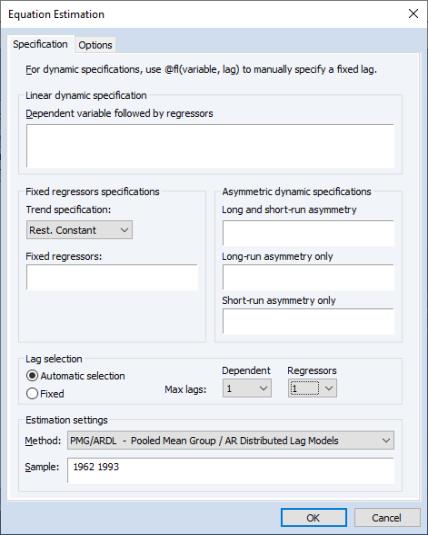
To estimate a Panel ARDL/PMG model in EViews, open the equation dialog by selecting , or by selecting and selecting PMG/ARDL from the Method dropdown menu. EViews 13 will then display the new ARDL estimation dialog:
While much of the dialog is familiar from earlier versions of EViews, notably different in the EViews 13 PMG dialog are additional entries in the corresponding to restricted intercept and trend specifications, and new edit fields for specifying . The upgrades allow for a wider range of long and short-term dynamics, while the latter fields support asymmetric variables in the PMG estimator:
EViews 13 also offers a number of new PMG diagnostics and tests to help you examine the dynamic behavior of your variables, the long-run properties of your specification, and the appropriateness of your model.
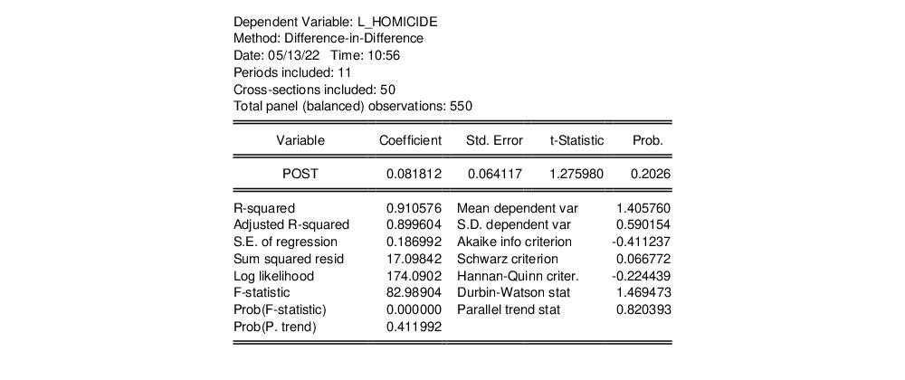
Difference-in-Difference Estimation
Difference-in-difference (DiD) estimation is a popular method of causal inference that allows estimation of the average impact of a treatment on individuals.
EViews 13 offers tools for estimation of the DiD model using the common two-way fixed-effects (TWFE) method, as well as post-estimation diagnostics of the TWFE model, such as those by Goodman-Bacon (2021), Callaway and Sant’Anna (2021), and Borusyak, Jaravel, and Spiess (2021).
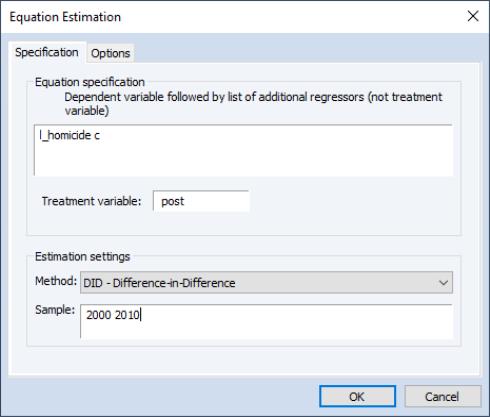
To estimate a DiD model in EViews, bring up the equation dialog by clicking on or from the main menu bar in your panel workfile. EViews will detect the presence of your panel structure and in place of the standard equation dialog will open the panel equation estimation dialog. Select DiD – Difference-in-Difference in the Method dropdown display the DiD dialog:
In the edit field you should enter the dependent variable followed by any exogenous regressors apart from the treatment variable.
The treatment variable should be entered in the edit field. The treatment series should be a binary variable indicating whether the individual has been treated (i.e., is 1 if the observation in a treatment group which is post-treatment date for that group, and 0 otherwise).
The tab contains a single edit field that allows you to change the default coefficient vector.
Click on to perform the difference-in-difference estimation and display the output:
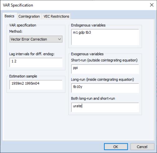
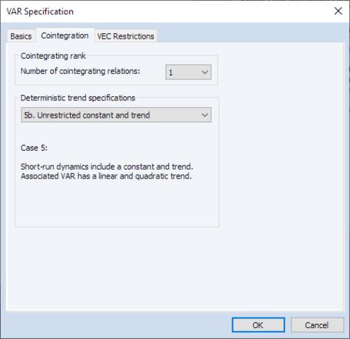
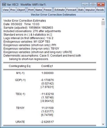
Enhanced VEC Estimation
Estimation of Vector Error Correction (VEC) models using reduced rank regression (RRR) has been a staple of EViews for several versions. Previous versions of EViews supported a variety of built-in specifications for deterministic trends, and allowed users to add unrestricted exogenous regressors to account for short-term dynamics.
One important limitation of the existing tools for VEC estimation was the inability of users to add arbitrary exogenous variables to the cointegrating relation since the set of admissible restricted regressors was limited to the endogenous variables and potentially an intercept, and possibly a linear trend term.
EViews 13 removes this limitation on restricted regressors and improves on the prior treatment of exogenous variables in two distinct ways:
• by providing new deterministic trend assumption presets which allow for more flexible specification of restricted and unrestricted deterministic coefficients, and
• by allowing users to add exogenous variables that are restricted to the cointegrating relation, variables that are unrestricted, and variables that in both the short and long-run equations, with an orthogonality assumption used to obtain the different coefficients.
To estimate a VEC using the new features, from the main application menu of an existing var object, click on the button to open the estimation dialog. Alternately, you may create a new VAR object by selecting Object/New Object... group, then selecting . Once the dialog appears, select in the dropdown menu to display the VEC estimation dialog:
The section of the main estimation dialog has fields for variables that are only, variables that are only, and variables that are .
Further, the dropdown on the tab offers additional predefined deterministic trend specifications.
Selecting a specification in which both intercept and trend are short-run only and clicking on produces estimates using the new deterministics:
• See
Var::ec in for updated command documentation.
Bayesian Time-varying Coefficient Vector Autoregression
The time-varying coefficients vector autoregression, or TVCVAR, is a nonlinear VAR model with coefficients that evolve smoothly over time. EViews 13 supports Bayesian TVCVAR, or BTVCVAR. The BTVCVAR is popular even among those who do not identify as Bayesian because the prior provides a convenient way to induce shrinkage in a model that needs it.
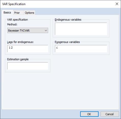
To estimate BTVCVAR in EViews, click on or run var in the command window. This will open the dialog. Select from the dropdown menu. The dialog should now have the , , and tabs.
Endogenous variables, lags, exogenous variables, and the estimation sample are set in the tab. Lags are required to be contiguous.
EViews gives users the option of setting aside a subset of the estimation sample for the purpose of specifying a prior distribution. The observations that go towards specifying the prior comprise the prior sample. The remaining observations make up the data sample, which is used to update the prior.
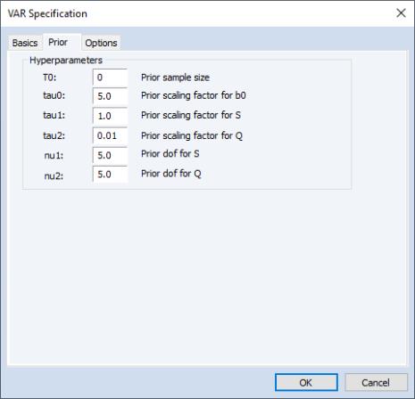
Prior hyper-parameters are set inside the tab. To help with setting the prior, EViews maps the BTVCVAR prior hyper-parameters to a set of six scalar quantities. Users set these scalars to specify a prior sample, control the variability of the time-varying coefficients, etc.
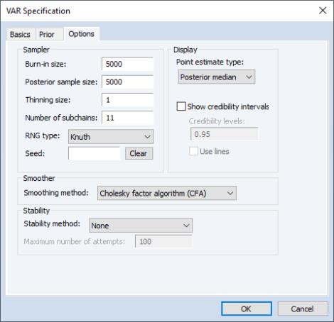
There are four categories in the tab: , , , and .
The options determine how the posterior sample is generated.
• The is the number of initial draws to discard. It is specified as a count. The burn-in process gives the underlying Markov chain time to converge to the posterior distribution.
• The is used to determine how many posterior draws are used to carry out post-updating procedures (estimation, forecasting, impulses responses analysis, etc.).
• The is used to thin the Markov chain. A thinning size of

indicates that every

-th draw is stored. For example, no thinning occurs when

is set to 1, and every other draw is stored when

is set to 2. By definition, thinning does not apply to burn-in draws.
• The field is used to set the random seed for the posterior simulator. EViews will generate a seed automatically if the user does not specify one. Click to clear the seed field.
• The field determines how many subchains are used when the posterior sample gets regenerated. Regeneration is typically much faster than initial generation since subchains can be run in parallel.
options determine what to report as estimation results. Users can pick either posterior median or posterior mean as their point estimate. The point estimate type selected here will be applied to the coefficients, the observation covariance matrix, and the errors. Users can also display equal-tailed credibility intervals (bands) at one or more credibility levels for the coefficients. To do so, check the box next to . Bands use shading by default. To use lines instead, check the box next to .
A simulation smoother can be selected from the dropdown menu under . EViews currently supports three simulation smoothers: the (CFA), the (KFS), and the method of (MMP). For more information, see McCausland, Miller, & Pelletier (2011) and the references therein.
To enforce stable VAR coefficients at each date within the data sample, select from the dropdown menu under . The threshold ensures that the sampler does not get stuck in an infinite loop in an attempt to obtain stable draws.
Once the BTVCVAR model has been specified, click on to run the posterior simulator. Progress is displayed in the bottom left corner of the EViews window. Once posterior simulation is complete, estimates and other statistics based on the posterior sample are computed.
Estimation results are presented in a spool-like object. The nodes under in the left pane are used for navigation. For example, clicking on the node will bring the summary table into focus. The checkboxes that appear below are used to show/hide coefficient series that are associated to specific endogenous variables, lags, and exogenous variables. For example, unchecking the box next to hides the coefficient series associated to the constant term in all graphs.
Cointegration Testing
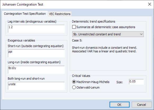
The introduction of new deterministic trend settings and exogenous variable support in EViews 13 VEC estimation offers corresponding improvements in cointegration testing in both group and var object settings.
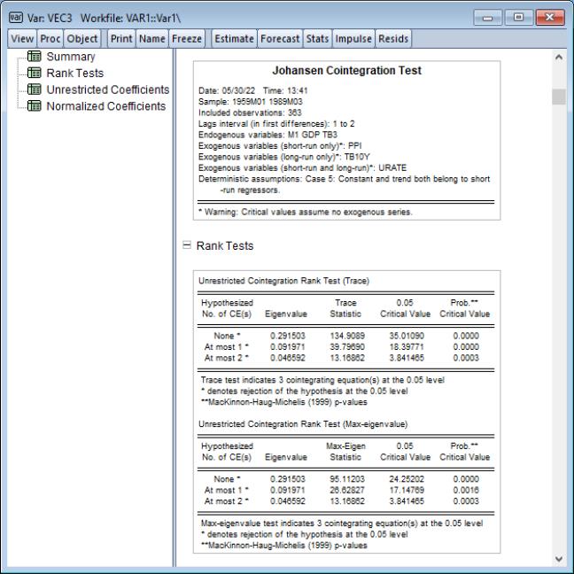
To perform a Johansen cointegration test to determine the rank that should be used in estimation of the VEC select , from a group window, or from an estimated VAR object window using. In the latter case, the test dialog will be pre-filled with the cointegration specification, if applicable:
All new settings allow you to specify new deterministic trend specifications with restricted constants and trends, and now allow you to specify exogenous variables that appear in the long-run cointegrating relation.
Diagnostics in ARDL
In addition to the support for nonlinear ARDL specifications, EViews 13 offers a number of new ARDL diagnostics. These diagnostics are designed to help you examine the dynamic behavior of your variables, the long-run properties of your specification, and the appropriateness of your model:
• Improved display tools make it easier to use the ARDL estimates to examine the short and long-run representations of the distributed lag regressors and cointegrating relationships. (
“Enhanced Presentation of ARDL Results”.)
• EViews now produces cumulative dynamic multipliers (CDM) graphs showing cumulative marginal contribution of an explanatory variable to the dependent variable (
“Cumulative Dynamic Multiplier Graphs”).
• Bounds tests are for cointegration are now available as a view of your ARDL equation (
“Bounds Tests”).
• You may evaluate symmetry restrictions on the coefficients of the asymmetric long and short-run regressors (
“Testing for Asymmetry”). Enhanced Presentation of ARDL Results
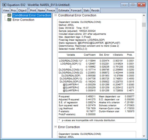
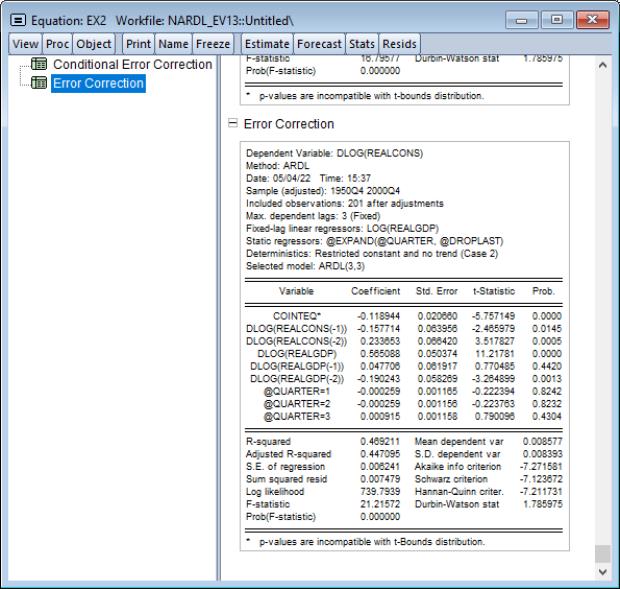
EViews 13 offers enhanced presentation of ARDL results, with an emphasis on highlighting the error correction results and the cointegrating relationship.
The new error correction spool output () shows two representations of the coefficients in the cointegrating relationship, allowing you to easily move between viewing the long-run relationship results in the Conditional Error Correction (CEC) and the Error Correction (EC) forms.
The CEC focuses on the natural division between long-run and short-run dynamics, with the former generated by regressors entering in levels/lags, and the latter by regressors in differences
while the EC representation uses the cointegrating relation to highlight the speed of adjustment to long-run equilibrium,
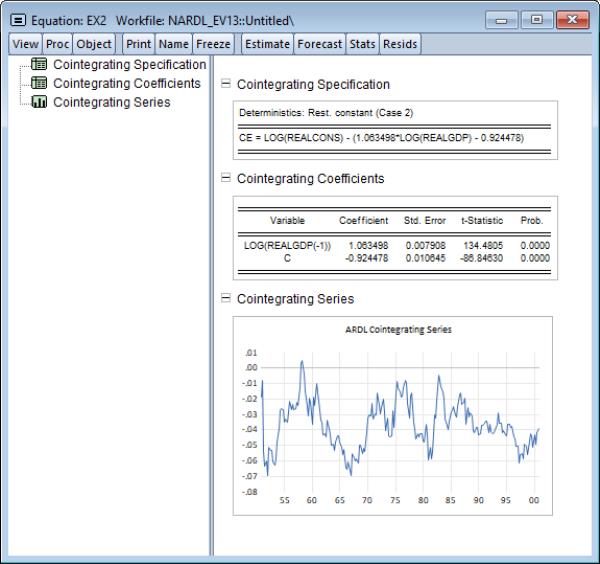
The new cointegrating relation spool view () lets you switch between viewing the specification, coefficient results, and a graphical display of the cointegrating relation.
Cumulative Dynamic Multiplier Graphs
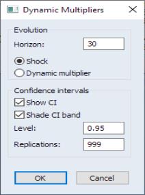
To display cumulative dynamic multiplier graphs for each of the explanatory variables in an EViews equation estimated using ARDL, click on
EViews will open a dialog containing display and computation settings:
• You may enter the horizon length

(number of periods to compute the multipliers) in the edit field.
• For NARDL models, you will be offered the opportunity to display confidence intervals for the computed absolute difference between the positive and negative components for a given regressor. CIs are not available for linear ARDL specifications.
You may check the to display the CIs, and to display the CIs as bands instead of lines. The edit field controls the size of the CI, and the governs how many replications to use in resampling for computing the CI.
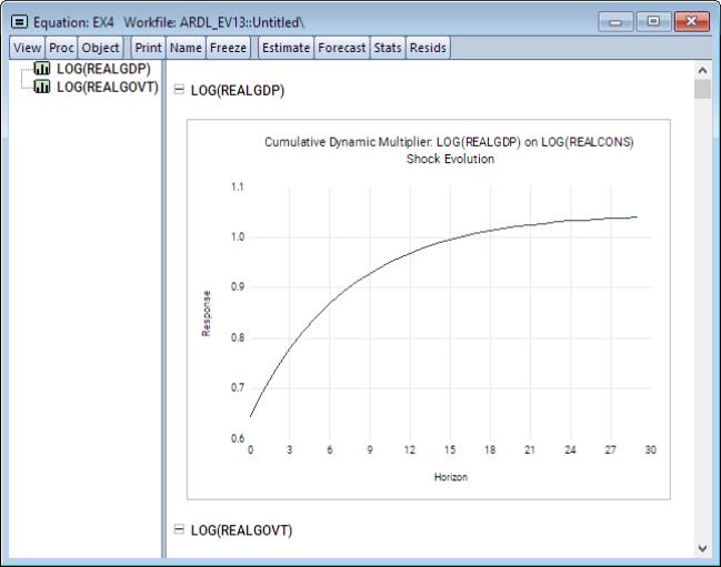
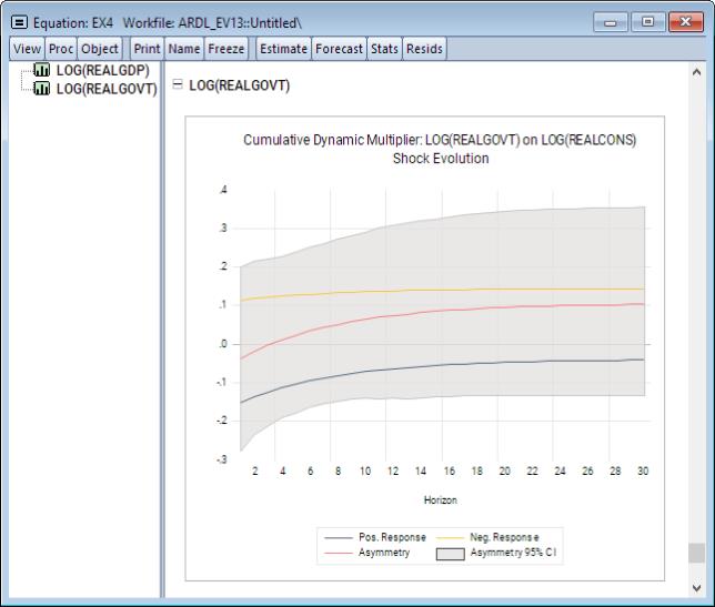
Click on to continue. EViews will open a spool view, with each node in the spool containing the CDM graph corresponding to one of the explanatory variables.
For symmetric linear models, each graph contains a CDM along with a dashed horizontal line denoting the long-run value.
For asymmetric nonlinear models, each graph will show the positive and negative responses and limit values, along with a line showing the absolute value of the difference between the two, and if requested, a CI for the absolute difference:
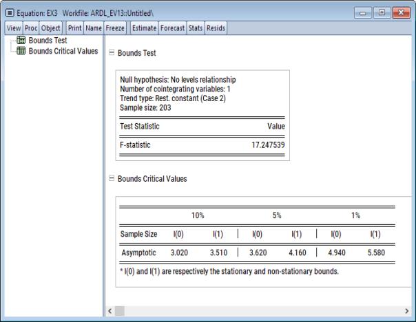
Bounds Tests
EViews 13 now performs Pesaran’s (2001) bounds tests for cointegration that are robust to whether variables of interest are

,

, or mutually cointegrated. These tests are formulated as standard
F-test or Wald tests of parameter significance in the cointegrating relationship of the Conditional Error Correction model for each cross-section.
To perform the bounds tests, click on . The results of the test performed are presented in the first table of a spool. Below the table of long run coefficient estimates are two additional tables, respectively titled as the

-Bounds Test and the

-Bounds Test.
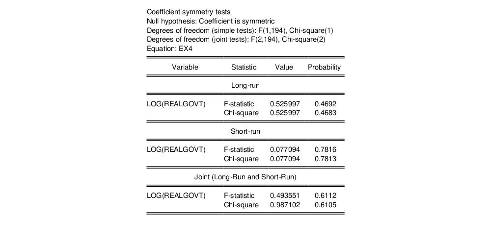
Testing for Asymmetry
The NARDL specification is quite general and can accommodate asymmetries in different combinations of short and long-run dynamics. From an estimated NARDL, you may test long-run symmetry restrictions and/or short-run symmetry restrictions.
To perform the symmetry tests on the estimated NARDL, click on from an estimated equation:
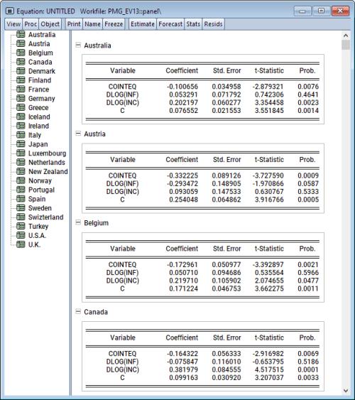
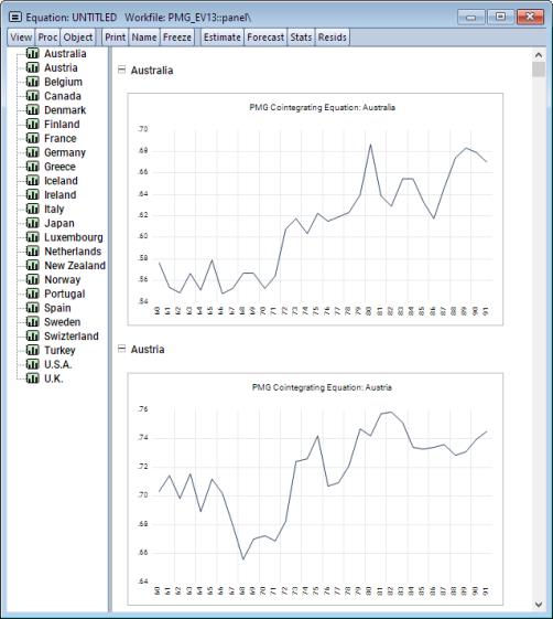
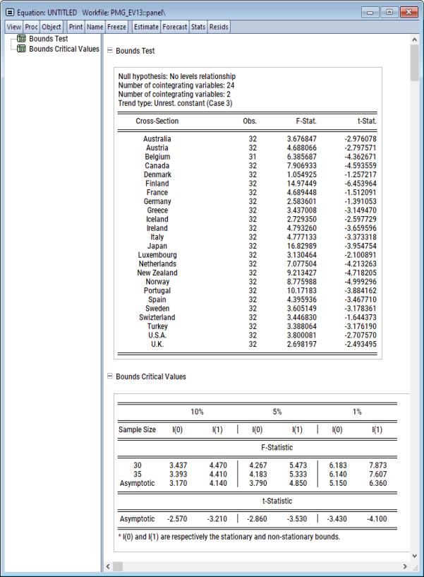
Diagnostics in Panel ARDL/PMG
EViews 13 features improved PMG diagnostics, including display of individual cross-section error correction equations coefficients and cointegrating series, cross-section specific bounds, Hausman tests for PMG coefficient similarity, and tests of symmetry restrictions:
• New views make it easier to use the PMG estimates to examine the short and long-run representations of the distributed lag regressors and cointegrating relationships. (
“Cross-sectional Cointegration Views”.)
• You may evaluate symmetry restrictions on the coefficients of asymmetric long and short-run regressors (
“Testing for Symmetry”).
• You may perform a Hausman-test of the similarity of the PMG estimator to the mean-group (MG) and dynamic fixed effects (DFE) estimators (
“Similarity Tests”).
For general discussion, see
“Linear and Nonlinear ARDL” in
User’s Guide II which discusses a variety of these features in non-panel settings
Cross-sectional Cointegration Views
The Error Correction Results view displays coefficient results for the error correction regressions for each cross-section. to display a spool of tables with results for each cross-section:
The Cointegrating Relations Plots view displays information about the error correction term

representing the cointegrating relation. Select to display a spool of plots for each cross-section:
Cross-sectional Bounds Tests
EViews 13 now performs Pesaran’s (2001) bounds tests for cointegration that are robust to whether variables of interest are

,

, or mutually cointegrated. These tests are formulated as standard
F-test or Wald tests of parameter significance in the cointegrating relationship of the Conditional Error Correction model for each cross-section.
To perform the bounds tests, click on . The results of the test performed on each cross-section are presented in the first table of a spool. Below the table of long run coefficient estimates are two additional tables, respectively titled as the

-Bounds Test and the

-Bounds Test.
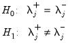
Testing for Symmetry
One can test for symmetry formally by performing the usual
t-test or
F-test of parameter equality. For example, testing for symmetry for a specific long-run (LR) variable, say

, is equivalent to the following hypothesis:
 | (0.1) |
To perform the symmetry test, select from the menu of a nonlinear asymmetric NARDL/PMG equation:
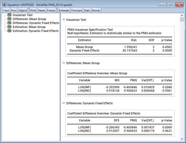
Similarity Tests
We may easily perform a Hausman test on the similarity of the PMG estimator to the mean-group (MG) and dynamic fixed effects (DFE) estimators. To conduct the test, click on :
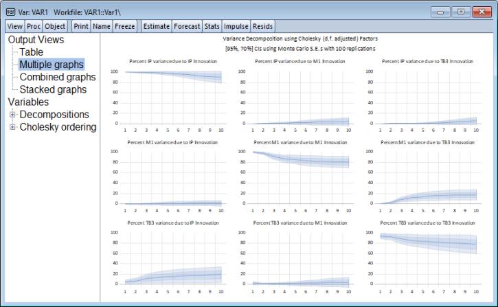
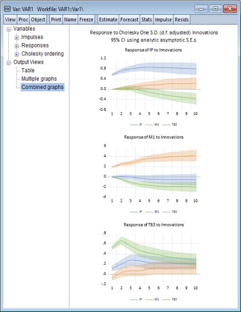
Enhanced Impulse Response Display
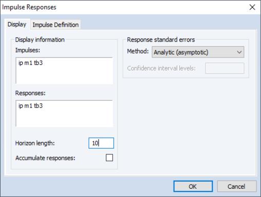
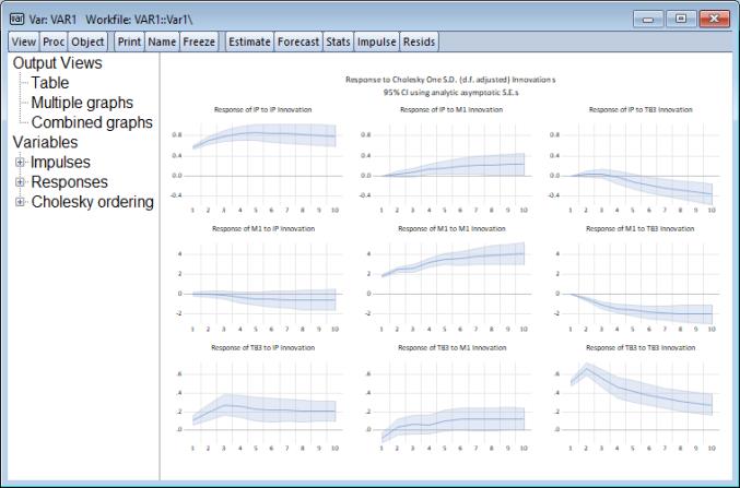
EViews 13 offers considerably more control over the computation and display of impulse response (and variance decomposition) confidence intervals. You may now display multiple confidence intervals with user-specified sizes in a single graph, and employ shading to improve the visibility of these intervals.
Recall that previous versions of EViews imposed important restrictions on the display of impulse response confidence intervals.
• First, for impulse-response confidence intervals computed using analytic or Monte Carlo standard errors, prior versions of EViews only allowed for the computation of +/- 2 standard error bands. There were no options for displaying different sized intervals, let alone for displaying different intervals in the same graph:
• Second prior EViews only allowed you to use dotted lines to display the confidence bands around the impulse-responses:
• Lastly, if you chose to display multiple impulses or responses in a combined graphs, confidence intervals were not available:
Fortunately, EViews 13 removes all three of these limitations.
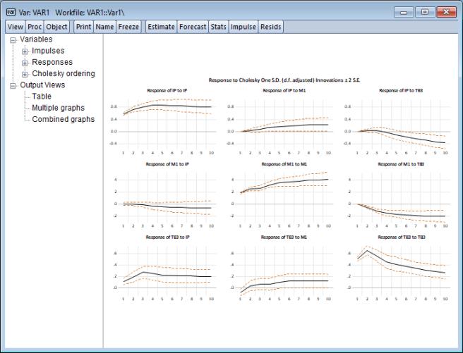
• First, by default, EViews 13 now uses shaded areas to depict confidence bands:
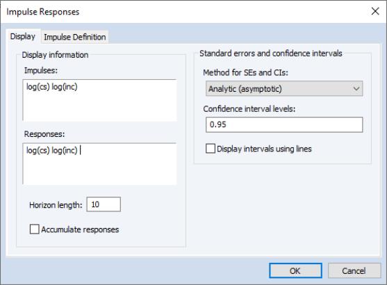
To display your graphs using the traditional lines, check the box next to in the impulse response dialog. If coming from the command line, you may use the uselines keyword in the impulse command options to display in the previous format.
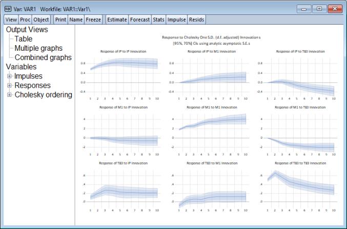
• Second, EViews 13 now lets users display analytic and monte carlo confidence intervals with one or more user-specified sizes:
When multiple shaded bands are displayed, EViews automatically uses the new EViews 13 line and shade transparency engine (
“Graph Line and Shade Transparency”) to display the bands using gradients:
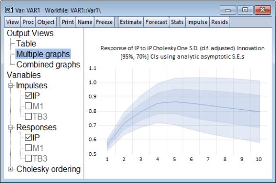
Using the selection interface to focus on the topmost left graph, better shows the shading:
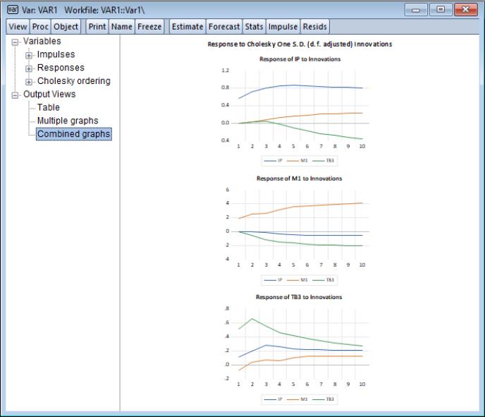
• Further, EViews 13 now allows you to display confidence intervals in the impulse-response combined graphs view:
All of the new shading and multiple band support is also provided for variance decomposition in multiple graph
and combined graph settings,
Forecast Sample Setting Commands
EViews 13 offers a small but surprisingly useful improvement in forecast sample setting.
Previously, forecasting via command generally required the user to first set the global smpl using a smpl statement prior to issuing the forecasting command.
For example, the following lines estimated the equation using one sample, and then forecast over two different samples,
smpl 1990q1 2010q4
equation eq1.ls y c x1 x2 x3
smpl 2011q1 2020q4
eq1.forecast fcst1
smpl 2008q3 2020q4
eq2.forecast fcst2
In this case, setting the global sample prior to equation forecasting was only mildly inconvenient. However, in some settings, particularly those involving non-equation forecasting where you are generating multiple forecasts and data, setting and resetting the global sample was inconvenient at best, and prone to error.
EViews 13 solves this problem by updating most forecast-generating commands to take a forecast sample information.
In this context, there are two types of forecasting procedures.
In the first set of procedures, the forecast sample is set independently of the remainder of the procedure. For these cases, EViews 13 offers an option to allow you to set the sample range pair directly using the option:
forcsmpl = smpl | Fit sample (optional). If forecast sample is not provided, the workfile sample will be employed. |
This option is available interactively and in commands for:
The second type of forecasting procedure sets the forecast sample one-period beyond a previously specified estimation sample, and then forecasting continues from that period onward until a forecast endpoint.
In this case, EViews 13 allows you to set the forecast sample in two distinct ways: by specifying the number of periods to forecast, or by specifying the forecast end date:
forclen=int | Number of periods to forecast. |
forc="date" | Specify the date of the forecast end point. |
These options are available interactively and in commands for:
Our earlier example changes from the commands
smpl 1990q1 2010q4
equation eq1.ls y c x1 x2 x3
smpl 2011q1 2020q4
eq1.forecast fcst1
smpl 2008q3 2020q4
eq2.forecast fcst2
to
smpl 1990q1 2010q4
equation eq1.ls y c x1 x2 x3
eq1.forecast(forcsmpl="2011q1 2020q4") fcst1
eq1.forecast(forcsmpl="2008q3 2020q4") fcst2