Estimating Quantile Regression in EViews
To estimate a quantile regression specification in EViews you may select or from the main menu, or simply type the keyword equation in the command window. From the main estimation dialog you should select . Alternately, you may type qreg in the command window.
EViews will open the quantile regression form of the dialog.
Specification
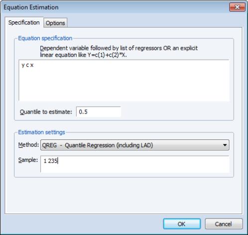
The dialog has two pages. The first page, depicted here, is used to specify the variables in the conditional quantile function, the quantile to estimate, and the sample of observations to use.
You may enter the using a list of the dependent and regressor variables, as depicted here, or you may enter an explicit expression. Note that if you enter an explicit expression it must be linear in the coefficients.
The edit field is where you will enter your desired quantile. By default, EViews estimates the median regression as depicted here, but you may enter any value between 0 and 1 (though values very close to 0 and 1 may cause estimation difficulties).
Here we specify a conditional median function for Y that depends on a constant term and the series X. EViews will estimate the LAD estimator for the entire sample of 235 observations.
Estimation Options
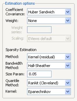
Most of the quantile regression settings are set using this page. The options on the left-hand side of the page control the method for computing the coefficient covariances, allow you to specify a weight series for weighted estimation, and specify the method for computing scalar sparsity estimates.
Quantile Regression Options
The dropdown menu labeled is where you will choose your method of computing covariances: computing covariances, using a method, or using resampling. By default, EViews uses the calculations which are valid under independent but non-identical sampling.
Just below the dropdown menu is an section , where you may define observations weights. The data will be transformed prior to estimation using this specification. (See
“Weighted Least Squares” for a discussion of the settings).
The remaining settings in this section control the estimation of the scalar sparsity value. Different options are available for different settings. For ordinary or bootstrap covariances you may choose either , , or as your sparsity estimation method, while if the covariance method is set to , only the and methods are available.
There are additional options for the bandwidth method (and associated size parameter if relevant), the method for computing empirical quantiles (used to estimate the sparsity or the kernel bandwidth), and the choice of kernel function. Most of these settings should be self-explanatory; if necessary, see the discussion in
“Sparsity Estimation” for details.
It is worth mentioning that the sparsity estimation options are always relevant, since EViews always computes and reports a scalar sparsity estimate, even if it is not used in computing the covariance matrix. In particular, a sparsity value is estimated even when you compute the asymptotic covariance using a Huber Sandwich method. The sparsity estimate will be used in non-robust quasi-likelihood ratio tests statistics as necessary.
Iteration Control
The iteration control section offers the standard edit field for changing the maximum number of iterations, a dropdown menu for specifying starting values, and a check box for displaying the estimation settings in the output. Note that the default starting value for quantile regression is 0, but you may choose a fraction of the OLS estimates, or provide a set of user specified values.
Bootstrap Settings
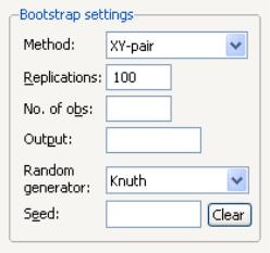
When you select in the dropdown, the right side of the dialog changes to offer a set of bootstrap options.
You may use the dropdown menu to choose from one of four bootstrap methods: , , , .See
“Bootstrapping” for a discussion of the various methods. The default method is .
Just below the dropdown menu are two edit fields labeled and By default, EViews will perform 100 bootstrap replications, but you may override this by entering your desired value. The edit field controls the size of the bootstrap sample. If the edit field is left blank, EViews will draw samples of the same size as the original data. There is some evidence that specifying a bootstrap sample size smaller than the original data may produce more accurate results, especially for very large sample sizes; Koenker (2005, p. 108) provides a brief summary.
To save the results of your bootstrap replications in a matrix object, enter the name in the edit field.
The last two items control the generation of random numbers. The dropdown should be self-explanatory. Simply use the dropdown to choose your desired generator. EViews will initialize the dropdown using the default settings for the choice of generator.
By default, the first time that you perform a bootstrap for a given equation, the edit field will be blank; you may provide your own integer value, if desired. If an initial seed is not provided, EViews will randomly select a seed value. The value of this initial seed will be saved with the equation so that by default, subsequent estimation will employ the same seed, allowing you to replicate results when re-estimating the equation, and when performing tests. If you wish to use a different seed, simply enter a value in the edit field or press the button to have EViews draw a new random seed value.
Estimation Output
Once you have provided your quantile regression specification and specified your options, you may click on to estimate your equation. Unless you are performing bootstrapping with a very large number of observations, the estimation results should be displayed shortly.
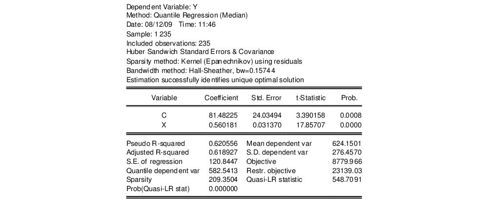
Our example uses the Engel dataset containing food expenditure and household income considered by Koenker (2005, p. 78-79, 297-307). The default model estimates the median of food expenditure Y as a function of a constant term and household income X.
The top portion of the output displays the estimation settings. Here we see that our estimates use the Huber sandwich method for computing the covariance matrix, with individual sparsity estimates obtained using kernel methods. The bandwidth uses the Hall and Sheather formula, yielding a value of 0.15744.
Below the header information are the coefficients, along with standard errors, t-statistics and associated p-values. We see that both coefficients are statistically significantly different from zero and conventional levels.
The bottom portion of the output reports the Koenker and Machado (1999) goodness-of-fit measure (pseudo R-squared), and adjusted version of the statistic, as well as the scalar estimate of the sparsity using the kernel method. Note that this scalar estimate is not used in the computation of the standard errors in this case since we are employing the Huber sandwich method.
Also reported are the minimized value of the objective function (“Objective”), the minimized constant-only version of the objective (“Restr. objective”), the constant-only coefficient estimate (“Quantile dependent var”), and the corresponding

form of the Quasi-LR statistic and associated probability for the difference between the two specifications (Koenker and Machado, 1999). Note that despite the fact that the coefficient covariances are computed using the robust Huber Sandwich, the QLR statistic assumes
i.i.d. errors and uses the estimated value of the sparsity.
The reported S.E. of the regression is based on the usual d.f. adjusted sample variance of the residuals. This measure of scale is used in forming standardized residuals and forecast standard errors. It is replaced by the Koenker and Machado (1999) scale estimator in the computation of the

form of the QLR statistics (see
“Standard Views and Procedures” and
“Quasi-Likelihood Ratio Tests”).
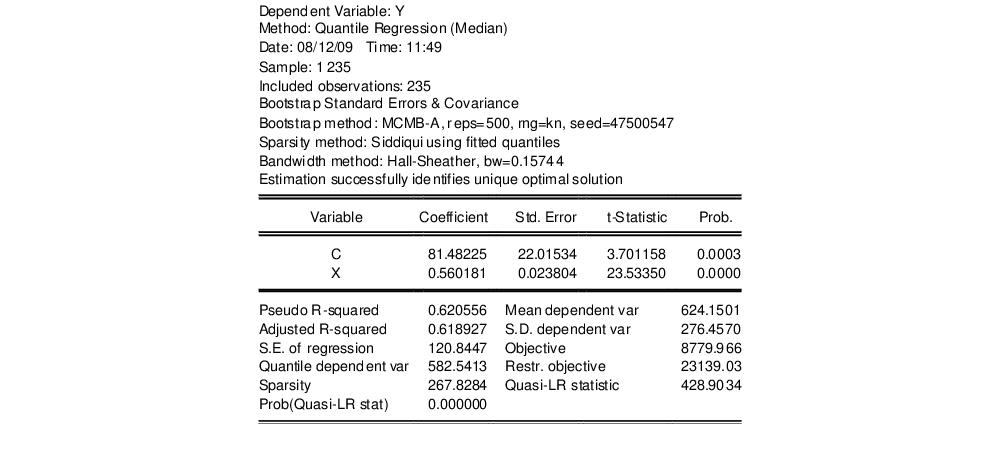
We may elect instead to perform bootstrapping to obtain the covariance matrix. Click on the button to bring up the dialog, then on to show the options tab. Select Bootstrap as the , then choose as the bootstrap method. Next, we increase the number of replications to 500. Lastly, to see the effect of using a different estimator of the sparsity, we change the scalar sparsity estimation method to . Click on to estimate the specification.
For the most part the results are quite similar. The header information shows the different method of computing coefficient covariances and sparsity estimates. The Huber Sandwich and bootstrap standard errors are reasonably close (24.03 versus 22.02, and 0.031 versus 0.024). There are moderate differences between the two sparsity estimates, with the Siddiqui estimator of the sparsity roughly 25% higher (267.83 versus 209.35), but this difference has no substantive impact on the probability of the QLR statistic.