Seasonal Adjustment
Time series observed at quarterly and monthly frequencies often exhibit cyclical movements that recur every month or quarter. For example, ice cream sales may surge during summer every year and toy sales may reach a peak every December during Christmas sales. Seasonal adjustment refers to the process of removing these cyclical seasonal movements from a series and extracting the underlying trend component of the series.
Seasonal adjustment procedures are only available in workfiles of the frequency they support. To seasonally adjust a series, click on Proc/Seasonal Adjustment in the series window toolbar and select the adjustment method from the submenu entries (JDemetra+, Census X-13, Census X-12, Tramo/Seats, MovReg, DSA Daily Seasonal Adjustment, STL Decomposition, or Moving Average Methods).
JDemetra+
JDemetra+ is an open-source seasonal adjustment and time-series analysis package created by the European Commission. EViews incorporates a subset of the functionality provided by JDemetra+ to perform X-13 style seasonal adjustment on monthly and quarterly data.
While the results provided JDemetra+ will often be numerically identical to the results provided by Census X-13 (for identical settings), JDemetra+ offers robust handling of missing or extreme values, and computes the seasonal adjustment with reduced processing time.
When accessed from within EViews, JDemetra+ will perform seasonal adjustment on the series over the current workfile sample. In contrast to other seasonal adjustment methods, JDemetra+ offers automatic handling of missing values:
• For internal missing values (those not at the start or end of the sample), JDemetra+ uses interpolation to fill in the missing values.
• For missing values at the beginning or end of the sample, EViews will adjust the start and end of the adjustment sample. While JDemetra+ permits extrapolation of missing values at the beginning and end of the sample, EViews simply the trims the sample to remove NAs before sending the data to JDemetra+.
To perform JDemetra+ seasonal adjustment in EViews, click on Proc/Seasonal Adjustment/JDemetra+... from the series window menu in a monthly or quarterly workfile. This will open the JDemetra+ tabbed dialog:
The first tab, Base specification allows you to choose one of the JDemetra+ preset specifications, as well as selecting which series to output into the workfile, and optionally specifying a suffix to be used in naming the output series.
• The X-13 spec: drop down menu specifies the preset specification. JDemetra+ offers a number of specifications with settings for the pre-treatment and decomposition steps of the seasonal adjustment:
| | | | |
X-11 | None | None | None | None |
RSA0 | None | None | None | Airline (0,1,1)(0,1,1) |
RSA1 | Automatic | AO/LS/TC | None | Airline (0,1,1)(0,1,1) |
RSA2c | Automatic | AO/LS/TC | TD2 (weekdays vs week-ends), Easter | Airline (0,1,1)(0,1,1) |
RSA3 | Automatic | AO/LS/TC | None | Automatic selection |
RSA4c | Automatic | AO/LS/TC | TD2 (weekdays vs week-ends), Easter | Automatic selection |
RSA5 | Automatic | AO/LS/TC | TD7 (7 day of week variables), Easter | Automatic selection |
For in-depth details of these specifications, we recommend browsing the JDemetra+
website (https://github.com/jdemetra).
• The Mode: dropdown specifies the X-11 decomposition mode that will be used. JDemetra+ only allows the user to specify the decomposition mode if no pre-adjustment is being performed, so this dropdown is only enabled when the X-11 default specification is selected.
• The Series output section specifies which of the output series from JDemetra+ will be exported to the workfile. By default, each output series will be created a name equal to that of the underlying series plus the type of series being created (e.g., if JDemetra+ is run on the series GDP, then the seasonally adjusted D11 series will be created with a name of GDP_D11). You can use the Naming suffix edit field to enter an additional suffix that will be appended to the series name before the output type (e.g., if you enter “_JD” as the Naming suffix then the D11 series for GDP will be created with a name of GDP_JD_D11).
The Regression tab of the dialog allows you to override some of the options set by the default specifications relating to the pre-adjustment regression step of X-13 style seasonal adjustment.
Selecting the X-13 specification on the Base specification tab will change the settings on this tab, but you can fine tune the default settings by using the options on this tab.
• The Transformation drop down menu specifies whether a log transformation should be applied to the underlying series before running the regression. Auto (Log/none) instructs JDemetra+ to automatically detect whether a log transform should be applied or not.
• The Check for outliers check box specifies whether JDemetra+ should automatically detect outliers. EViews' implementation of JDemetra+ supports only the Additive Outlier (AO), Level Shift (LS), and Temporary Change (TC) types of outliers, and when the option is checked, JDemetra+ will detect for all three types simultaneously.
• Trading days sets the type of calendar effects used in the pre-adjustment regression. These effects consist of created variables with the count of the number of days in each period compared to the number of reference days. The options are:
None | Do not include calendar effects. |
TD7 | Create 6 calendar variables. The first counts the number of Mondays in the month/quarter compared to the number of Sundays. The second counts the number of Tuesdays compared to the number of Sundays, and so on. |
TD4 | Create 3 calendar variables. The first counts the number of days from Monday to Thursday compared with the number of Sundays, the second counts the number of Fridays compared with the number of Sundays, the third counts Saturdays compared with Sundays. |
TD3c | Create 2 calendar variables. The first counts the number of days from Monday to Thursday compared to the number of Sundays, the second counts the number of Fridays and Saturdays compared to the number of Sundays. |
TD3 | Create 2 calendar variables. The first counts the number of days from Monday to Friday compared with the number of Sundays, the second counts the number of Saturdays compared with the number of Sundays. |
TD2 | Create 1 calendar variable which is the number of week days (Mon-Fri) compared to the number of Saturday and Sundays. |
TD2c | Create 1 calendar variables which is the number of days from Monday to Saturday compared with the number of Sundays. |
User variables | Include user-provided calendar variables only. |
If User variables is selected as the trading day type, you must specify series to use as calendar variables on the User Regressors tab.
• The Test: dropdowns specify whether JDemetra+ should test for the inclusion of trading day or Easter effects. Selecting Remove tells JDemetra+ to include the effects, but test for removal. Add tells JDemetra+ to not include the effects by default, but test to include. None tells JDemetra+ to always include the effects.
• The Include Leap Year adjustment and Include Easter checkboxes control whether additional adjustments are made to the calendar effects for the impact of leap years and Easter. The Auto-adjust checkbox specifies whether JDemetra will automatically determine whether to drop the leap-year adjustment.
The ARIMA tab provides options for the estimation of the ARIMA model in the pre-adjustment step:
• The ARIMA Method section selects the method used to specify the ARIMA model to be estimated. None instructs JDemetra+ to not estimate an ARIMA model at all.
If Manual is selected, you can enter a specific ARIMA order in (p, d, q)(P, D, Q) notation, where p is the AR order, d is the differencing level, q is the MA order, P is the seasonal AR order, D is the seasonal differencing level, and Q is the seasonal MA order.
If X-11 Auto is selected, JDemetra+ will use its default X-11 selection routine to select the most appropriate ARIMA order.
• The Forecast ARIMA model checkbox instructs JDemetra+ to forecast the ARIMA model beyond the end of the series. The number of periods forecasted can be changed using the Forecast length edit field. Forecasting the ARIMA model allows JDemetra+ to provide forecasts of the final seasonally adjusted series and seasonal factors. Note forecasts will only be imported into EViews if the workfile range covers the period of the forecast.
The User Regressors tab of the dialog supports providing user-provided exogenous series to the pre-adjustment ARIMA/regression models.
Clicking on the Add button brings up a dialog asking you to type in the name of the workfile variable that you would like to include as a regressor:
You may enter any valid EViews series name or expression, such as "X" or "log(X)", or "@pch(X)" in the edit field. You may also type in a space delimited list to add multiple series at once.
The drop down menu should be used to specify a regressor type for the variable you are including (i.e., , , , etc.). Changing the type of the regressors changes the exact impact that series has on the final seasonal adjustment calculation. The JDemetra+ documentation has details on the exact calculations.
If you selected User Variables as the Trading Days type, you must add at least one user-regressor with a type of Calendar/TradingDay.
Example
The workfile, "X13_Macro.wf1" includes a series called UNRATENSA which contains monthly non-seasonally adjusted US unemployment data from January 2005 to June 2012. We will use this series to demonstrate the user of JDemetra+ seasonal adjustment in EViews. We will later use the same series to demonstrate X-13 seasonal adjustment.
We will perform simple X-11 based seasonal adjustment on this series without any pre-adjustment regression options being set. To do so open the UNRATENSA series and click on to open the JDemetra+ dialog.
Simple X-11 adjustment is one of the pre-set JDemetra+ defaults, so we change the X-13 spec: dropdown to X-11. We'll elect to store the seasonally adjusted values in the workfile, and enter “_x11” in the edit field:
Clicking to display the JDemetra+ graph output:
The output is split into five graphs. The top graph displays the original unadjusted series. The second displays the decomposed trend line, the third the seasonal/cyclical factors, the fourth the irregular/residual component, and finally graph displays the seasonally adjusted values. It should be noted that this simple X-11 adjustment via JDemetra+ will give numerically identical results to using EViews’ implementation of Census X-13 using the default settings.
Census X-13
EViews offers an easy-to-use front-end for working with the U.S. Census Bureau’s X-13 seasonal adjustment tools. The publicly available Census X-13ARIMA-SEATS seasonal adjustment program “X13.EXE” is included with your copy of EViews and is pre-installed in your EViews directory.
In addition to providing a wide range of new features, X-13 is capable of performing updated versions of X-11/X-12 or TRAMO/SEATS ARIMA seasonal adjustment. For backwards compatibility, EViews still supports the older X-11, X-12 and TRAMO/SEATS routines, but we recommend that you use the newer X-13 routines.
When you perform X-13 seasonal adjustment, EViews carries out the following steps:
• write out a specification file and data files for the series
• execute the X-13 program in the background, using the contents of the specification file
• read back the output file and saved data into your EViews workfile
The remainder of this section offers a brief description of the EViews interactive interface to
X-13ARIMA-SEATS. EViews provides a general command interface that also supports X-13 features not available via the dialogs (see
Series::x13).
Users who require a detailed discussion of the X-13 procedures and capabilities should consult the Census Bureau documentation. The full documentation for the Census program, X-13ARIMA-SEATS Reference Manual, can be found in the “docs” subdirectory of your EViews installation directory in the PDF file “X-13 Reference Manual.pdf”.
Note that X-13 combines standard least-squares regression, ARIMA, and regARIMA estimation, with X-11 or SEATS seasonal adjustment. To simplify matters, we will refer to regression, ARIMA, and regARIMA estimation collectively as the “ARIMA” or “ARIMA regression” portion of the X-13 seasonal adjustment procedure.
To perform X-13 seasonal adjustment, select from the series window menu in a quarterly or monthly workfile. EViews will open a tree structured dialog containing branches for setting options for variables, ARIMA estimation and forecasting, seasonal adjustment, and output.
X-13 Variable Options
The X-13ARIMA-SEATS procedure allows you to perform ARIMA regression prior to the seasonal adjustment step. The first branch of the X-13 dialog includes options for defining the source series and exogenous variables used in the ARIMA step.
Transform
The Transform settings allow you to transform the source series and regressors before fitting the ARIMA model.
When you click on the entry you will be prompted to choose a transformation method. You may choose between no transformation (), or a natural log (), Box-Cox (), logistic (), or automatically selected () transformation.
The
Auto option chooses between no transformation and a log transformation based on the Akaike information criterion. The
Logit option transforms the series

to

and is defined only for series with values that are strictly between 0 and 1. For the
Box-Cox option, you must provide the parameter value

for the transformation:
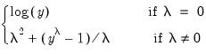 | (11.38) |
for

. See “Transform” (Section 7.18) of the
X-13ARIMA-SEATS Reference Manual for further details.
X-13 built-in regressors
The X-13 built in regressors page lets you specify any of the X-13 built-in regressors for the ARIMA regression model:
You may use the drop-down menus to add a constant, seasonal variables (such as seasonal dummies), trading-day effects, holidays or outliers to the ARIMA model. Only one type of seasonal variable and one type of trading-day effect can be selected, but multiple holidays or outliers are supported. To add a holiday or outlier, simply specify the variable to add in the appropriate section of the dialog and click on the button.
As you make selections or add variables, the X-13 Specification box will display the corresponding X-13 text specification. You may manually add, edit, or remove entries in this box and the dialog settings will change to reflect your entries, where relevant. For more details on the built-in variable types, see the “Variables” part of Section 7.13 (“Regression”), and Table 7.27 of the X-13ARIMA-SEATS Reference Manual.
X-13 user-defined regressors
The User-defined regressors page allows non-X-13 built-in variables to be used as regressors in the ARIMA model:
Clicking on the Add button brings up a dialog asking you to type in the name of the workfile variable that you would like to include as a regressor:
You may enter any valid EViews series name or expression, such as “X” or “log(X)”, or “@pch(X)” in the edit field.
The dropdown menu should be used to specify a regressor type for the variable you are including (i.e., , , , ). Knowledge of the variable type may be used in internal calculations. Note that you may define up to five different holiday types and you may include multiple variables of a given holiday type. If your regressor variable does not fit in any of the specific categories, you should designate it as .
Once you have added user-defined regressors you may choose whether X-13 will perform model-selection for the specified variables using AIC-based selection or Chi-square tests by checking one or both of the checkboxes.
For additional details on the elements of the User-defined regressors page, see Section 7.13 of the X-13ARIMA-SEATS Reference Manual, notably the entries for “user”, “usertype”, “aictest” and “chi2test”.
Automatic Outliers
The Automatic outliers entry allows specification of automatic outlier detection routines.
The controls in the Outlier types box may be used to select which type of outliers to detect, and the range of dates over which to detect them.
The Selection procedure box lets you specify the method used to select outliers ( or and associated critical values against which the absolute t-statistics for the tests will be compared. You may enter a single critical value to apply to all of the outlier types, or a list of critical values, one for each type. The default settings, which are outlined in Table 7.22 of the X-13ARIMA-SEATS Reference Manual, vary with the number of observations.
Details of the outlier types and the selection procedures can be found in Section 7.11 of the X-13ARIMA-SEATS Reference Manual. The “DETAILS” section has a detailed description of the two different selection methods, “addone” (One at a time) and “addall” (All at once).
X-13 ARIMA Options
The ARIMA options branch is used to specify the ARIMA portion of the model, and to as provide access to basic estimation and forecasting options.
ARIMA Model
You will specify the ARIMA model to be estimated on the Model page, using the radio buttons in section:
• The default setting, None, tells X-13 not to include an ARIMA specification. (Note that SEATS seasonal adjustment requires an ARIMA specification, so you may not select None setting if you wish to use SEATS.)
• If you select , , or , the dialog will change to show you the settings corresponding to your choice. We discuss each of these methods in turn.
Manual
If you select Manual as the ARIMA method, you will be prompted to specify the exact ARIMA specification in “(p, d, q) (P, D, Q)” format, where the “(p, d, q)” are the standard ARIMA components (for the AR, differencing and MA orders, respectively) and the “(P, D, Q)” are the seasonal ARIMA components at the workfile frequency.:
The first edit field, labeled , should be used to enter the text specification of the model, For example, to estimate a model with an AR(1), first differencing, an MA(1), a seasonal AR(1), no seasonal differencing and no seasonal MA terms, you would enter:
(1, 1, 1)(1, 0, 0)
The edit field allows you to specify starting values for the AR coefficients in the ARIMA model. By default this field is left blank, meaning that X-13 default values will be used for starting values. If you wish to specify starting values, you must enter a starting value for every AR term (including seasonal AR terms), separated by a comma.
In addition, note that:
• Individual terms may be left blank between commas to indicate that the X-13 default should be used for that specific term. For example, for a (2, 1, 1)(1, 0, 0) model, you may enter “0.2, , 0.3” to indicate that a starting value of 0.2 should be used for the first AR term, the X-13 default starting value should be used for the second AR term, and 0.3 should be used for the seasonal AR term.
• You may specify that a specific term should be fixed at its starting value (not estimated) by including an “f” after its value. For example entering “0.2f, , 0.3” means that the first AR term is fixed at 0.2, the second AR term uses the default X-13 starting value, and the seasonal AR term has a starting value of 0.3.
The edit field allows you to specify starting values for the MA terms in the ARIMA specification. The syntax for this edit field is the same as the one used for setting the AR starting coefs.
For more information on the specification of a specific ARIMA model and setting the starting values, see Section 7.1 (ARIMA) of the X-13ARIMA-SEATS Reference Manual.
X-11 Auto
If you choose X-11 Auto as the ARIMA Method, X-13 will automatically select the best ARIMA model using an algorithm from X-11-ARIMA. You will be prompted to specify a set of models from which to choose and a set of selection options.
The X-11-ARIMA model selection algorithm requires that you specify a set of ARIMA models from which to choose. The drop-down menu in the section offers a choice between three methods for specifying the candidate models: By list, With limits, or By file.
When you select one of these entries, the remaining portion of the dialog will change to show the corresponding options:
• If you select By list, you will be prompted to specify candidate models in a list box on the right side of the dialog.
Each line should contain a candidate specification specified in “(p, d, q) (P, D, Q)” format. The list box will be pre-filled with a default set of specifications to test.
• If you select With limits, you will be prompted to set the maximum order of each term in the ARIMA model.
EViews will build up the set of candidate models by choosing every combination of orders up to the maximums you select. Note that X-11-ARIMA may not be able to identify the preferred model if you set the maximum number of terms to large values.
• If you select , you will be prompted to specify a file on disk containing a list of candidate models:
For details of the specification of the file, see the DETAILS part of Section 7.12 (Pickmdl) of the X-13ARIMA-SEATS Reference Manual.
The Options group box provides access to important X-11 Auto options.
• Forecast Mode specifies whether both forecasts and backcasts (Forwards and back) or only forecasts (Forecast only) will be used during the model selection process.
• The Forecast Errors option allows you to select whether or forecast errors are used during the model selection.
• Stopping Method allows you select the model selection routine. If you choose Once 1 model is found, X-13 will stop searching through the list of available models as soon as it finds one that meets the selection criteria. If you select Check all models, X-13 will select the best model out of all models that meet the selection criteria.
The section allows you to specify the limit values for forward, and (if relevant) backward selection.
The X11 selection procedure evaluates models using the forecast and backcast errors or forecast errors alone. A model is accepted if the absolute average percentage error of the forecast is less than the limit, and likewise for the backcast, if relevant.
Additional details on these options may be found in Section 7.12 (“Pickmdl”) of the X-13ARIMA-SEATS Reference Manual.
TRAMO Auto
Selecting TRAMO Auto as the ARIMA Method instructs X-13 to choose the best ARIMA model using an algorithm from TRAMO/SEATS.
The Differencing and ARMA sections of the dialog let you specify the maximum order of differencing and ARMA terms. Note that the Auto/Fixed radio buttons allow you to set the level of differencing at a fixed value or to choose the level automatically.
The Options box contains settings for the TRAMO model selection routine:
• The Check significance of constant term check box specifies whether TRAMO will test for statistical significance of the constant term in the ARIMA model.
• Allow mixed models determines whether TRAMO will allow mixed ARIMA models (i.e. models with both AR and MA terms) or not.
• Reject out of sample forecasts tells TRAMO to test the out-of-sample forecast errors for the final three years of data, and to suppress forecasts if the forecast error surpasses the given limit.
• The option specifies whether TRAMO will automatically accept the default model “(0, 1, 1)(0, 1, 1)” and ignore all other models if the default passes a Ljung-Box Q-statistic test.
ARIMA Estimation
The Estimation page lets you specify basic estimation options for the ARIMA with regressors model.
The Likelihood method drop-down allows you to specify whether an exact or a conditional likelihood is used for estimation and forecasting. The accompanying edit fields allow you to specify a maximum number of iterations and convergence tolerance.
You may use the edit field to specify a sample for the estimation of the model. By default the estimation sample is the same as the sample used for seasonal adjustment (i.e. the current workfile sample), but you may specify a contiguous sub-sample of the seasonal adjustment sample.
ARIMA Forecasting
The Forecast page offers options for forecasting or backcasting from the chosen model once it has been estimated.
You may specify a forecast and backcast length (
i.e., the number of observations to be forecasted or backcasted), and you may instruct X-13 to make an adjustment to the forecasts to reflect the fact that they are generated from a log-normal distribution whenever a log-transformation is specified (see
“Transform”).
Note that specifying a forecast or backcast length that produces data outside of the current workfile range will not produce an error, but any observations outside of the workfile range will not be brought into EViews.
X-13 Seasonal Adjustment Options
The Seasonal Adjustment branch of the dialog contains the options for the actual seasonal adjustment process undertaken by X-13.
You may use the radio buttons in the section to select either X-11 or SEATS based seasonal adjustment, or you may chose to perform no seasonal adjustment so that X-13 simply estimates the specified ARIMA regression model.
If you specify a seasonal adjustment method, EViews will display a set of options. The two checkboxes allow you to instruct X-13 to append one year of forecasted and/or backcasted values to certain output series (e.g., the seasonal factors D10, if performing X-11 adjustment and the seasonal factors S10, if performing SEATS adjustment), and to display the results in the table output.
For a full list of series that can be forecasted/backcasted see the “appendfcst” and “appendbcst” entries in Section 7.19 of the X-13ARIMA-SEATS Reference Manual (if performing X-11 seasonal adjustment) and the “appendfcst” and “appendbcst” entries in Section 7.14 of the X-13ARIMA-SEATS Reference Manual (if performing SEATS).
The remaining portion of the dialog will show options for the X-11 and the SEATS seasonal adjustment methods.
• If you specify X-11 as the seasonal adjustment method you will be presented with a few X-11 based options.
The Method drop-down menu lets you set the seasonal adjustment decomposition method. You may choose between , , , , or , where the latter lets X-13 choose the mode depending upon the transformation (if any) given on the Variables branch.
The Trend filter box allows you to choose the Henderson trend moving average used for the final trend-cycle. You can let X-13 choose a value for you, or you may specify a fixed length (note only odd integers between 1 and 101 can be used).
The Seasonal filter drop-down specifies the type of seasonal moving average to employ. By default, X-13 will choose the type of seasonal filter automatically, but you may, if you prefer, choose a specific filter.
See Table 7.51 of the X-13ARIMA-SEATS Reference Manual for details on each filter type.
• Selecting SEATS as the seasonal adjustment method brings up SEATS based options.
You may select whether to decompose the trend-cycle into a long term cycle using the Hodrick-Prescott filter by selecting the Use HP filter option.
The Do not allow stationary seasonal models option tells X-13 to disallow adjustment of any seasonal model with no differencing. If this option is selected and a stationary seasonal ARIMA model is specified, X-13 will replace the seasonal ARIMA component with a (0, 1, 1) specification.
The Ljung-Box Q limit sets the limit SEATS uses to test whether the provided ARIMA model is of acceptable quality.
X-13 Force Options
The Force section provides the ability to force annual totals of the adjusted series to match those of the original series. X-13 provides two methods for forcing the totals; the original Denton method of X-11, and a newer regression benchmarking method of Cholette and Dagum (1994) as adapted by Quenneville, Cholette, Huot, Chiu, and Fonzo (2004).
Selecting the check box instructs X-13 to force the annual totals, and enables the Options section of the dialog. Those options allow you to change the method of forcing from Denton to the regression method using the combo-box, switch the whether the ratio or difference of the annual totals is used with the combo-box, and change the target series from the original data to an adjusted version of the original data with the combo-box.
The and fields can be used to fine tune the parameters of the forcing algorithms, and the checkbox is used to instruct X-13 to use rounded data rather than the exact data.
More information on the X-13 force option can be found in Section 7.6 of the X-13ARIMA-SEATS Reference Manual.
X-13 Output Options
The Output section allows you to set which output series will be added to the workfile.
When performing either X-11 or SEATS seasonal adjustment, you may elect to output the seasonally adjusted data (called D11 in X-11 short name terminology, and S11 in SEATS), the trend component (D12, S12), seasonal factors (D10, S10) or the irregular component (D13, S13) by selecting the corresponding check boxes in the section.
If you chose SEATS as the seasonal adjustment method, the section of the dialog offers the option of saving the transitory component (S14), and the section allows you to save the forecasted values of the seasonally adjusted series (AFD), trend (TFD), transitory component (YFD), seasonal factors (SFD).
Each of these output series will be imported into EViews with a name given by the original series name plus an underscore followed by the X-13 short name. For example, if your original series is called GDP, the X-11 seasonal factors will be added to the workfile with the name GDP_D10.
If you chose to perform forecasting by setting the options (see
“ARIMA Forecasting”), you will also be given the choice to output the forecasted values and confidence bounds of the forecasted values. The point forecasts will be brought into the workfile with a name suffix of “_f”, and the lower and upper bounds will have suffixes of “_fl” and “fu” respectively.
You may save other X-11 or SEATS output series to your workfile by typing their short names into the Other seasonal adjustment output series edit field. A full list of available output series, and their corresponding short names, can be found in Table 7.46 in Section 7.19 of the X-13ARIMA-SEATS Reference Manual (if performing X-11), and Tables 7.30 and 7.31 in Section 7.14 (if performing SEATS).
If you wish to save the X-13 specification file as a text object in your workfile, enter a name in the file box. Saving the specification file lets you reuse or modify the specification for further use (note that you can specify X-13 via the command line using a text object in the workfile).
Lastly, X-13 is capable of generating both text and html output. Check the checkbox to view the X-13 results as html or uncheck the box to view the results in text. While the html output provides easier navigation tools and is aesthetically more pleasing, it cannot be frozen and therefore cannot viewed again without recalculating. The text output on the other hand, can be frozen into a text object and referred to a later point in time.
Example
As an example of using the EViews X-13 proc, we will seasonally adjust monthly employment data obtained from the Federal Reserve Economic Data (FRED) database. The EViews workfile, “X13_Macro.wf1” contains monthly non-seasonally adjusted US unemployment data from January 2005 to June 2012 in a series called UNRATENSA. We will perform two types of seasonally adjustment: X-11 with automatic ARIMA selection performed using X-11-Auto, and SEATS based with automatic ARIMA selection performed using TRAMO.
To perform X-11 based seasonal adjustment with automatic ARIMA selection using X-11-Auto, open the UNRATENSA series and click on Proc/Seasonal Adjustment/Census X-13. EViews will display the X-13 dialog”
• Note that this example will not be using any exogenous variables, transformations or outliers in the model so skip the settings in the branch of the tree structure
• Click on the ARIMA branch to display the ARIMA options. Select X-11 Auto as the ARIMA Method, and leave the remaining options at their default values.
• Open the Seasonal Adjustment branch and select X-11 as the Seasonal adjustment method.
• Select the Output branch and check all four of the Final series output boxes so that EViews will import the seasonally adjusted values, the trend values (D12), the seasonal factors (D10) and the irregular components (D13) into the workfile.
After you click on OK, EViews will run the X-13ARIMA-SEATS program using the specified settings and will display the text output produced by the program in the series window. In addition, EViews will save the four output series UNRATENSA_D10, UNRATENSA_D11, UNRATENSA_D12 and UNRATENSA_D13 in the workfile.
UNRATENSA_D11 contains the final seasonally adjusted series. Select this series along with the original UNRATENSA, right-click and , then select and click on to display a line graph of the adjusted and unadjusted series:
The smoothed series UNRATENSA_D11 clearly exhibits less seasonally volatility than the original series UNRATENSA.
Displaying the graph views of the remaining series lets you view the individual components of the smoothing. For example, showing a graph of UNRATENSA_D12 enables you to see the trend component.
For comparison purposes, we perform SEATS based seasonal adjustment with automatic outlier detection on the same data. Select Proc/Seasonal Adjustment/Census X-13 from the series menu to display the X-13 dialog:
• Open the branch of the dialog. Instruct EViews to perform automatic outlier selection by checking all four of the Outlier types boxes (, , , ). Leave the remaining settings at their defaults.
• Open the ARIMA branch of the tree, select the node, and select TRAMO Auto as the ARIMA Method. Leave all other options at their defaults.
• Open the Seasonal Adjustment branch, select SEATS as the Seasonal adjustment method, and select the Append forecasts option.
• Finally, switch to the Output branch, select the first four Final series output boxes to instruct EViews to import the seasonally adjusted values, the trend values, the seasonal factors, and the irregular components into the workfile. Note that by default the forecasted seasonal adjustment values (AFD) is selected in the Forecast output box.
• Click on OK to run X-13 with these settings and bring the five output series from X-13 to our workfile. Note that EViews will save the results in the new series UNRATENSA_S10, UNRATENSA_S11, UNRATENSA_S12 and UNRATENSA_S13, and UNRATENSA_AFD.
We may open up a group object containing the seasonally adjusted series, UNRATENSA_S11, along the X-11 seasonally adjusted series UNRATENSA_D11 by selecting the three series, right-clicking and selecting group. Extend the workfile sample by two years (24 months) by issuing the command
smpl @first 2012m06+24
select and click on to display a line graph of the two adjusted and one unadjusted series:
Notice that the SEATS seasonally adjusted series, UNEMPNSA_S11, closely tracks the X-11 adjusted series, UNEMPNSA_D11, with both offering a seasonally smoother version of the original series.
Also note that since we used the Append forecasts to instruct SEATS to append two years of forecasts to the final seasonally adjusted value, the UNEMPSNA_S11 series continues until June 2014.
Census X12
EViews provides a convenient front-end for accessing the U.S. Census Bureau’s X12 seasonal adjustment program from within EViews. The X12 seasonal adjustment program X12A.EXE is publicly provided by the Census and is installed in your EViews directory.
When you request X12 seasonal adjustment from EViews, EViews will perform all of the following steps:
• write out a specification file and data file for the series.
• execute the X12 program in the background, using the contents of the specification file.
• read back the output file and saved data into your EViews workfile.
The following is a brief description of the EViews menu interface to X12. While some parts of X12 are not available via the menus, EViews also provides a more general command interface to the program (see
x12).
Users who desire a more detailed discussion of the X12 procedures and capabilities should consult the Census Bureau documentation. The full documentation for the Census program, X12-ARIMA Reference Manual, can be found in the “docs” subdirectory of your EViews installation directory in the PDF files “Finalpt1.PDF” and “Finalpt2.PDF”.
To call the X12 seasonal adjustment procedure, select from the series window menu. A dialog will open with several tabs for setting the X12 options for seasonal adjustment, ARIMA estimation, trading day/holiday adjustment, outlier handling, and diagnostic output.
It is worth noting that when you open the X12 dialog, the options will be set to those from the previously executed X12 dialog. One exception to this rule is the outlier list in the tab, which will be cleared unless the previous seasonal adjustment was performed on the same series.
Seasonal Adjustment Options
specifies the form of the seasonal adjustment decomposition. A description of the four choices can be found in pages 75-77 of the
X12-ARIMA Reference Manual. Be aware that the Pseudo-additive method must be accompanied by an ARIMA specification (see
“ARIMA Options” for details on specifying the form of your ARIMA).
Note that the multiplicative, pseudo-additive, and log-additive methods do not allow for zero or negative data.
The drop-down box allows you to select a seasonal moving average filter to be used when estimating the seasonal factors. The default setting is an automatic procedure based on the moving seasonality ratio. For details on the remaining seasonal filters, consult the X12-ARIMA Reference Manual. To approximate the results from the previous X11 program’s default filter, choose the X11-default option. You should note the following:
• The seasonal filter specified in the dialog is used for all frequencies. If you wish to apply different filters to different frequencies, you will have to use the more general X12 command language described in detail in
x12.
• X12 will not allow you to specify a

seasonal filter for series shorter than 20 years.
• The Census Bureau has confirmed that the X11-default filter option does not produce results which match those obtained from the previous version of X11. The difference arises due to changes in extreme value identification, replacement for the latest values, and the way the end weights of the Henderson filter is calculated. Earlier versions of EViews provided (historical) X11 routines as a separate procedure (see
“Census X11 (Historical)”), but the programs do not run on 64-bit operating systems and are no longer supported.
The settings allow you to specify the number of terms in the Henderson moving average used when estimating the trend-cycle component. You may use any odd number greater than 1 and less than or equal to 101. The default is the automatic procedure used by X12.
You must provide a base name for the series stored from the X12 procedure in the edit box. To save a series returned from X12 in the workfile, click on the appropriate check box. The saved series will have the indicated suffix appended to the base name. For example, if you enter a base name of “X” and ask to save the seasonal factors (“_SF”), EViews will save the seasonal factors as X_SF.
You should take care when using long base names, since EViews must be able to create a valid series using the base name and any appended Census designations. In interactive mode, EViews will warn you that the resulting name exceeds the maximum series name length; in batch mode, EViews will create a name using a truncated base name and appended Census designations.
The dialog only allows you to store the four most commonly used series. You may, however, store any additional series as listed on Table 6-8 (p. 74) of the
X12-ARIMA Reference Manual by running X12 from the command line (see
x12).
ARIMA Options
The X12 program also allows you to fit ARMA models to the series prior to seasonal adjustment. You can use X12 to remove deterministic effects (such as holiday and trading day effects) prior to seasonal adjustment and to obtain forecasts/backcasts that can be used for seasonal adjustment at the boundary of the sample. To fit an ARMA, select the ARIMA Options tab in the X12 Options dialog and fill in the desired options.
The setting allows you to transform the series before fitting an ARMA model. The
Auto option selects between no transformation and a log transformation based on the Akaike information criterion. The
Logistic option transforms the series

to
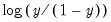
and is defined only for series with values that are strictly between 0 and 1. For the
Box-Cox option, you must provide the parameter value

for the transformation
 | (11.39) |
See the “transform spec” (p. 60–67) of the X12-ARIMA Reference Manual for further details.
allows you to choose between two different methods for specifying your ARIMA model. The Specify in-line option asks you to provide a single ARIMA specification to fit. The X12 syntax for the ARIMA specification is different from the one used by EViews and follows the Box-Jenkins notation “(p d q)(P D Q)” where:
p | nonseasonal AR order |
d | order of nonseasonal differences |
q | nonseasonal MA order |
P | (multiplicative) seasonal AR order |
D | order of seasonal differences |
Q | (multiplicative) seasonal MA order |
The default specification “(0 1 1)(0 1 1)” is the seasonal IMA model:
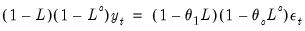 | (11.40) |
Here are some other examples (

is the lag operator):
(1 0 0) | |
(0 1 1) | |
(1 0 1)(1 0 0) | where  for quarterly data and  for monthly data. |
You can skip lags using square brackets and explicitly specify the seasonal order after the parentheses:
See the X12-ARIMA Reference Manual (p. 110–114) for further details and examples of ARIMA specification in X12. Note that there is a limit of 25 total AR, MA, and differencing coefficients in a model and that the maximum lag of any AR or MA parameter is 24 and the maximum number of differences in any ARIMA factor is 3.
Alternatively, if you choose Select from file, X12 will select an ARIMA model from a set of possible specifications provided in an external file. The selection process is based on a procedure developed by Statistics Canada for X11-ARIMA/88 and is described in the X12-ARIMA Reference Manual (p. 133). If you use this option, you will be asked to provide the name of a file that contains a set of possible ARIMA specifications. By default, EViews will use a file named X12A.MDL that contains a set of default specifications provided by Census (the list of specifications contained in this file is given below).
To provide your own list in a file, the ARIMA specification must follow the X12 syntax as explained in the ARIMA Specification section above. You must specify each model on a separate line, with an “X” at the end of each line except the last. You may also designate one of the models as a “default” model by marking the end of a line with an asterisk “*” instead of “X”; see p. 133 of the X12-ARIMA Reference Manual for an explanation of the use of a default model. To ensure that the last line is read, it should be terminated by hitting the return key.
For example, the default file (X12A.MDL) provided by X12 contains the following specifications:
(0 1 1)(0 1 1) *
(0 1 2)(0 1 1) x
(2 1 0)(0 1 1) x
(0 2 2)(0 1 1) x
(2 1 2)(0 1 1)
There are two additional options for Select from file. Select best checks all models in the list and looks for the model with minimum forecast error; the default is to select the first model that satisfies the model selection criteria. Select by out-of-sample-fit uses out-of-sample forecast errors (by leaving out some of the observations in the sample) for model evaluation; the default is to use within-sample forecast errors.
The option allows you to include pre-specified sets of exogenous regressors in your ARIMA model. Simply use the checkboxes to specify a constant term and/or (centered) seasonal dummy variables. Additional predefined regressors to capture trading day and/or holiday effects may be specified using the Trading Day/Holiday tab. You can also use the Outlier tab to capture outlier effects.
Trading Day and Holiday Effects
X12 provides options for handling trading day and/or holiday effects. To access these options, select the tab in the dialog.
As a first step you should indicate whether you wish to make these adjustments in the ARIMA step or in the X11 seasonal adjustment step. To understand the distinction, note that there are two main procedures in the X12 program: the X11 seasonal adjustment step, and the ARIMA estimation step. The X11 step itself consists of several steps that decompose the series into the trend/cycle/irregular components. The X12 procedure may therefore be described as follows:
• optional preliminary X11 step (remove trading day/holiday effects from series, if requested).
• ARIMA step: fit an ARIMA model (with trading/holiday effects, if specified) to the series from step 1 or to the raw series.
• X11 step: seasonally adjust the series from step 2 using backcasts/forecasts from the ARIMA model.
While it is possible to perform trading day/holiday adjustments in both the X11 step and the ARIMA step, Census recommends against doing so (with a preference to performing the adjustment in the ARIMA step). EViews follows this advice by allowing you to perform the adjustment in only one of the two steps.
If you choose to perform the adjustment in the X11 step, there is an additional setting to consider. The checkbox instructs EViews to adjust only if warranted by examination of the Akaike information criterion.
It is worth noting that in X11, the significance tests for use of trading day/holiday adjustment are based on an
F-test. For this, and a variety of other reasons, the X12 procedure with “X11 settings” will not produce results that match those obtained from historical X11. To obtain comparable results, you must use the historical X11 procedure (see
“Census X11 (Historical)”).
Once you select your adjustment method, the dialog will present additional adjustment options:
• — There are two options for trading day effects, depending on whether the series is a flow series or a stock series (such as inventories). For a flow series, you may adjust for day-of-week effects or only for weekday-weekend contrasts. Trading day effects for stock series are available only for monthly series and the day of the month in which the series is observed must be provided.
• — Holiday effect adjustments apply only to flow series. For each holiday effect, you must provide a number that specifies the duration of that effect prior to the holiday. For example, if you select 8, the level of daily activity changes on the seventh day before the holiday and remains at the new level until the holiday (or a day before the holiday, depending on the holiday).
Note that the holidays are as defined for the United States and may not apply to other countries. For further details, see the X12-ARIMA Reference Manual, Tables 6–15 (p. 94) and 6–18 (p. 133).
Outlier Effects
As with trading day/holiday adjustments, outlier effects can be adjusted either in the X11 step or in the ARIMA step (see the discussion in
“Trading Day and Holiday Effects”). However, outlier adjustments in the X11 step are done only to robustify the trading day/holiday adjustments in the X11 step. Therefore, in order to perform outlier adjustment in the X11 step, you must perform trading day/holiday adjustment in the X11 step. Only additive outliers are allowed in the X11 step; other types of outliers are available in the ARIMA step. For further information on the various types of outliers, see the
X12-ARIMA Reference Manual, Tables 6–15 (p. 94) and 6–18 (p. 133).
If you do not know the exact date of an outlier, you may ask the program to test for an outlier using the built-in X12 diagnostics.
Diagnostics
This tab provides options for various diagnostics. The Sliding spans and Historical revisions options test for stability of the adjusted series. While Sliding spans checks the change in adjusted series over a moving sample of fixed size (overlapping subspans), Historical revisions checks the change in adjusted series over an increasing sample as new observations are added to the sample. See the X12-ARIMA Reference Manual for further details and references of the testing procedure. You may also choose to display various diagnostic output:
• Residual diagnostics will report standard residual diagnostics (such as the autocorrelation functions and Q-statistics). These diagnostics may be used to assess the adequacy of the fitted ARIMA model. Note that this option requires estimation of an ARIMA model; if you do not provide an ARIMA model nor any exogenous regressors (including those from the or tab), the diagnostics will be applied to the original series.
• Outlier detection automatically detects and reports outliers using the specified ARIMA model. This option requires an ARIMA specification or at least one exogenous regressor (including those from the or tab); if no regression model is specified, the option is ignored.
• Spectral plots displays the spectra of the differenced seasonally adjusted series (SP1) and/or of the outlier modified irregular series (SP2). The red vertical dotted lines are the seasonal frequencies and the black vertical dashed lines are the trading day frequencies. If you observe peaks at these vertical lines it is an indication of inadequate adjustment. For further details, see Findley et al. (1998, section 2.1). If you request this option, data for the spectra will be stored in a matrix named seriesname_sa_sp1 and seriesname_sa_sp2 in your workfile. The first column of these matrices are the frequencies and the second column are 10 times the log spectra at the corresponding frequency.
X11/X12 Troubleshooting
The currently shipping versions of X11 and X12 as distributed by the Census have the following limitation regarding directory length. First, you will not be able to run X11/X12 if you are running EViews from a shared directory on a server which has spaces in its name. The solution is to map that directory to a letter drive on your local machine. Second, the temporary directory path used by EViews to read and write data cannot have more than four subdirectories. This temporary directory used by EViews can be changed by selecting in the main menu. If your temporary directory has more than four subdirectories, change the Temp File Path to a writeable path that has fewer subdirectories. Note that if the path contains spaces or has more than 8 characters, it may appear in shortened form compatible with the old DOS convention.
Tramo/Seats
Tramo (“Time Series Regression with ARIMA Noise, Missing Observations, and Outliers”) performs estimation, forecasting, and interpolation of regression models with missing observations and ARIMA errors, in the presence of possibly several types of outliers. Seats (“Signal Extraction in ARIMA Time Series”) performs an ARIMA-based decomposition of an observed time series into unobserved components. The two programs were developed by Victor Gomez and Agustin Maravall.
Used together, Tramo and Seats provide a commonly used alternative to the Census X12 program for seasonally adjusting a series. Typically, individuals will first “linearize” a series using Tramo and will then decompose the linearized series using Seats.
EViews provides a convenient front-end to the Tramo/Seats programs as a series proc. Simply select and fill out the dialog. EViews writes an input file which is passed to Tramo/Seats via a call to a .DLL, and reads the output files from Tramo/Seats back into EViews (note: since EViews uses a new .DLL version of Tramo/Seats, results may differ from the older DOS version of the program).
Since EViews only provides an interface to an external program, we cannot provide any technical details or support for Tramo/Seats itself. Users who are interested in the technical details should consult the original documentation Instructions for the User which is provided as a .PDF file in the Docs/TramoSeats subdirectory of your EViews directory.
Dialog Options
The Tramo/Seats interface from the dialog provides access to the most frequently used options. Users who desire more control over the execution of Tramo/Seats may use the command line form of the procedure as documented in
tramoseats.
The dialog contains three tabs. The main tab controls the basic specification of your Tramo/Seats run.
• : You can choose either to run only Tramo or you can select the checkbox to run both. In the latter case, EViews uses the input file produced by Tramo to run Seats. If you wish to run only Seats, you must use the command line interface.
• : You may set the number of periods to forecast outside the current sample. If you choose a number smaller than the number of forecasts required to run Seats, Tramo will automatically lengthen the forecast horizon as required.
• : Tramo/Seats is based on an ARIMA model of the series. You may choose to fit the ARIMA model to the level of the series or to the (natural) log of the series, or you select . This option automatically chooses between the level model and the log transformed model using results from a trimmed range-mean regression; see the original Tramo/Seats documentation for further details.
• : You may either specify the orders of the ARIMA model to fit or ask Tramo to search for the “best” ARIMA model. If you select in the dropdown menu and specify the order of all of the ARIMA components, Tramo will use the specified values for all components where the implied ARIMA model is of the form:
with seasonal frequency

. When you fix the order of your ARIMA you should specify non-negative integers in the edit fields for

,

,

,

,

, and

.
Alternatively, if you select , Tramo will search for the best ARMA model for differenced data of the orders specified in the edit fields.
You can also instruct Tramo to choose all orders. Simply choose or to have Tramo find the best ARIMA model subject to limitations imposed by Tramo. The two options differ in the handling of complex roots. Details are provided in the original Tramo/Seats documentation.
Warning: if you choose to run Seats after Tramo, note that Seats has the following limit on the ARIMA orders:

,

,

,

,

,

.
• : To save series output by Tramo/Seats in your workfile, provide a valid base name and check the series you wish to save. The saved series will have a postfix appended to the basename as indicated in the dialog. If the saved series contains only missing values, it indicates that Tramo/Seats did not return the requested series see
“Trouble Shooting”.
If Tramo/Seats returns forecasts for the selected series, EViews will append them at the end of the stored series. The workfile range must have enough observations after the current workfile sample to store these forecasts.
If you need access to series that are not listed in the dialog options, see
“Trouble Shooting”.
• : You may provide your own exogenous series to be used by Tramo. These must be a named series or a group in the current workfile and should not contain any missing values in the current sample and the forecast period.
If you selected a trading day adjustment option, you have the option of specifying exogenous series to be treated as a holiday series. The specification of the holiday series will depend on whether you chose a weekday/weekend adjustment or a 5-day adjustment. See the original Tramo/Seats documentation for further details.
If you are running Seats after Tramo, you must specify which component to allocate the regression effects. The Tramo default is to treat the regression effect as a separate additional component which is not included in the seasonally adjusted series.
EViews will write a separate data file for each entry in the exogenous series list which is passed to Tramo. If you have many exogenous series with the same specification, it is best to put them into one group.
• : These options are intended for monthly data; see the original Tramo/Seats documentation for details.
• : You may either ask Tramo to automatically detect possible outliers or you can specify your own outlier but not both. If you wish to do both, create a series corresponding to the known outlier and pass it as an exogenous series.
Similarly, the built-in intervention option in Tramo is not supported from the dialog. You may obtain the same result by creating the intervention series in EViews and passing it as an exogenous series. See the example below.
The original Tramo/Seats documentation provides definitions of the various outlier types and the method to detect them.
After you click , the series window will display the text output returned by Tramo/Seats. If you ran both Tramo and Seats, the output from Seats is appended at the end of Tramo output. Note that this text view will be lost if you change the series view. You should freeze the view into a text object if you wish to refer to the output file without having to run Tramo/Seats again.
It is worth noting that when you run Tramo/Seats, the dialog will generally contain the settings from the previous run of Tramo/Seats. A possible exception is the user specified outlier list which is cleared unless Tramo/Seats is called on the previously used series.
Comparing X12 and Tramo/Seats
Both X12 and Tramo/Seats are seasonal adjustment procedures based on extracting components from a given series. Methodologically, X12 uses a non-parametric moving average based method to extract its components, while Tramo/Seats bases its decomposition on an estimated parametric ARIMA model (the recent addition of ARIMA modelling in X12 appears to be used mainly to identify outliers and to obtain backcasts and forecasts for end-of-sample problems encountered when applying moving average methods.)
For the practitioner, the main difference between the two methods is that X12 does not allow missing values while Tramo/Seats will interpolate the missing values (based on the estimated ARIMA model). While both handle quarterly and monthly data, Tramo/Seats also handles annual and semi-annual data. See the sample programs in the directory for a few results that compare X12 and Tramo/Seats.
Trouble Shooting
Error handling
As mentioned elsewhere, EViews writes an input file which is passed to Tramo/Seats via a call to a .DLL. Currently the Tramo/Seats .DLL does not return error codes. Therefore, the only way to tell that something went wrong is to examine the output file. If you get an error message indicating that the output file was not found, the first thing you should do is to check for errors in the input file.
When you call Tramo/Seats, EViews creates two subdirectories called Tramo and Seats in a temporary directory. This temporary directory is taken from the global option (note that long directory names with spaces may appear in shortened DOS form). The Temp File Path can be retrieved in a program by a call to
@temppath@temppath.
The Tramo input file written by EViews will be placed in the subdirectory Tramo and is named serie. A Seats input file written by Tramo is also placed in subdirectory Tramo and is named Seats.itr.
The input file used by Seats is located in the Seats subdirectory and is named serie2. If Seats is run alone, then EViews will create the SERIE2 file. When Tramo and Seats are called together, the Tramo file Seats.itr is copied into serie2.
If you encounter the error message containing the expression “output file not found”, it probably means that Tramo/Seats encountered an error in one of the input files. You should look for the input files serie and serie2 in your temp directories and check for any errors in these files.
Retrieving additional output
The output file displayed in the series window is placed in the Output subdirectory of the Tramo and/or Seats directories. The saved series are read from the files returned by Tramo/Seats that are placed in the Graph subdirectories. If you need to access other data files returned by Tramo/Seats that are not supported by EViews, you will have to read them back into the workfile using the read command from these Graph subdirectories. See the PDF documentation file for a description of these data file formats.
Warning: if you wish to examine these files, make sure to read these data files before you run the next Tramo/Seats procedure. EViews will clear these subdirectories before running the next Tramo/Seats command (this clearing is performed as a precautionary measure so that Tramo/Seats does not read results from a previous run).
MoveReg Weekly Seasonal Adjustment
EViews offers a front-end interface to the U.S. Bureau of Labor’s MoveReg weekly seasonal adjustment program. Most seasonal adjustment routines, including the U.S. Census Bureau’s X-11, X-12 and X-13 packages, require the data be sampled at a monthly or quarterly frequency. However, many economic series are sampled on a weekly basis, meaning that these seasonal adjustment techniques cannot be used. The MoveReg program rectifies this gap by providing a seasonal adjustment method aimed directly at weekly data.
Similar to many of the other seasonal adjustment methods in EViews, the MoveReg routine performs the following steps:
• Write out a specification and data file for the series and the provided options.
• Execute the MoveReg program in the background using the created specification and data files.
• Read the output back into the EViews workfile.
To perform MoveReg seasonal adjustment, open the series and select EViews will then open a dialog allowing you to specify the options for the MoveReg procedure:
The dialog has three tabs. The first tab, , provides the basic MoveReg specification options, as well some output options.
To change the width of the detrending filter used by the MoveReg procedure, use the edit field. The and fields can be used to change the AR parameter and variance ratio term of the ARMA specification respectively. To modify the number of trigonometric terms used in the regression, change the field. Note that this is the total number of terms, including both sine and cosine terms. Since the number of sine and cosine must be equal, this number must be an even positive integer.
The area specifies the names of the series that will be imported into the EViews workfile. To change the name of the seasonally adjusted data and the seasonal factors, use the and edit fields respectively. If you have specified outliers on the tab, you can choose to import the outlier factors by entering a name into the field. Similarly, if you have specified holidays in the tab, you can import them by providing a name in the field.
The tab allows specification of both additive and level shift outliers:
To add an additive outlier, enter the outlier’s date into the edit field. Note you can enter the date either as a week number followed by the year, or as an explicit date in “YYYY/MM/DD” format. EViews will convert a date into week number year format. Once you have entered the date, click the button to add the outlier to the outlier list. If you would like to remove an added outlier, select it and then click the button.
Level shift outliers can be specified in an identical manner to the additive ouliers.
Holidays can be specified on the tab:
MoveReg allows for two types of holidays – built in special holidays or user-defined events.
To select a built in holiday, use the combo box to choose one of the pre-defined holidays, then enter a weighting scheme in the edit field below the combo. The weighting scheme should be specified as defined by the MoveReg application – the first digit should be the number of weights (the length of the holiday effect, in weeks), the second should be position of the holiday in the weights, and the final digits should be the weights themselves. The digits are separated by a space.
For example, entering “1 1 1” means the holiday lasts one observation (week), the position of the holiday is the first weight, and that weight has a value of 1. “3 2 1 2 1” means the holiday last three weeks, where the second weight is the holiday itself. The week before the holiday date has a weight of one, the week of the holiday a weight of two, and the week following the holiday date has a weight of one.
Once you have selected the holiday and entered its weighting scheme, you can click the button to add it to the list. If you would like to remove a previously added holiday, you can select it and click the button.
The edit field can be used to specify your own holidays/events. Simply enter the name of one or more series in the workfile containing binary information on whether an observation is a holiday/event or not.
Troubleshooting
The MoveReg procedure can be very sensitive to the specification of holidays. In particular:
• If a user event is provided, data for that event must extend two years beyond the last date in the adjustment sample. If data is not provided, MoveReg will fail. If a user event series is provided, and data is not available for two years (either because of NAs in the series, or because the workfile range does not extend for two years beyond the current sample), EViews will fill the event series with zeros for the missing observations.
• MoveReg will only forecast seasonal adjustment factors for two years beyond the adjustment sample if holidays or user events are included in the specification.
• MoveReg will often fail if sparse (mainly zeros with few ones) user events are included, or if none are included.
If holidays are required, we strongly recommend always including at least one user-event with regular ones.
An Example
As an example we will perform MoveReg seasonal adjustment on U.S. weekly unemployment initial claims (non-seasonally adjusted) data between the 30th December 1989 and 22nd October 2016.
We first obtain the data by creating a weekly workfile with those dates and fetching the data from the FRED database, with the following EViews commands:
wfcreate w 12/30/1989 10/22/2016
dbopen(type=fred)
fetch(db=fred) icnsa
We open the ICNSA series by double clicking on it, and then view a graph of the series by clicking on , and then selecting :
These data exhibit strong seasonal patterns. To remove this seasonality we perform MoveReg seasonal adjustment by clicking on To begin we perform the adjustment without allowing for holiday or outlier effects, and so keep all dialog options at their defaults:
Clicking performs the adjustment, producing the following output:
The first part of the spooled output provides a brief description of what we did, including the name of the underlying series, the name of the created seasonally adjusted series, the number of observations that were used, and the options that we chose.
The second part provides a graph showing the original, unadjusted series (in red in our case), alongside the produced seasonally adjust series (in green). It is clear that for our data the MoveReg procedure did a good job of removing the seasonal effects.
The remainder of the spooled output contains information and output provided by the MoveReg procedure itself. This information can be useful in performing diagnostics on the procedure.
We continue our analysis by adding in some outlier and holiday options to the procedure. Clicking brings up the dialog again. Since we will be adding outliers and holidays, and wish to see their effects, we enter series names into their output boxes:
Switching to the tab we believe there may be an additive outlier in the second week of September in 2008 (the Lehman Brother’s bankruptcy), and one for 9/11 2001:
(here we have not yet clicked the button to enter the 9/11 outlier).
On the tab we enter a Christmas holiday effect. We believe the holiday effect of Christmas will last 5 weeks, 3 weeks before Christmas, the week of the 25th, and the week after. The week of and the week after will have slightly greater weights than the weeks before:
(again we have not yet clicked in this screenshot).
Clicking produces similar output:
The summary information at the top again describes the options we chose, including the outlier and holiday specification. EViews has translated the outlier dates into week year format in the output.
The graph of the adjusted values looks very similar to the original (indeed comparison of the two adjusted series indicates that the addition of outliers and holidays led to only a 0.1% difference).
EViews now offers a new graph displaying the outlier and holiday factors as part of the spooled output:
The remaining nodes of the spool contain the text of the Census program output.
Daily Seasonal Adjustment
Daily Seasonal Adjustment (DSA) models daily time series data that contains three distinct seasonalities—a day-of-the-week (DoW) effect, a day-of-the-month (DoM) effect, and a day-of-the-year (DoY) effect, as well as potential holiday or event/calendar effects.
EViews offers an implementation of the seasonal adjustment of daily time series algorithm of Ollech (2021).
Background
Although the original Ollech (2021) algorithm is designed for 7-day week daily data, EViews’ implementation handles both 7 and 5-day week daily data.
7-day Seasonal Adjustment
The seasonal adjustment process of 7-day weekly data with DSA can be broken down into five stages:
• Stage 1: Adjusting for the day-of-the-week effect using STL decomposition.
• Stage 2: Remove holiday and calendar effects using ARIMA modeling.
• Stage 3: Adjusting for the day-of-the-month effect using STL decomposition.
• Stage 4: Adjusting for the day-of-the-year effect using STL decomposition.
• Stage 5: Combining the adjustments and performing any out-of-sample forecasts.
Each of these stages may further be broken down into individual steps.
Stage 1: Day-of-the-week adjustment
The first stage adjusts for the DoW effect by performing STL decomposition on the original data with a periodicity set to 7.
Stage 2: Holiday and calendar effects
The holiday and calendar effects are modeled using a seasonal ARIMA process. This can both model the impact of known events, or detect and model unknown effects using outlier detection.
Following Ollech (2021), EViews approximates the yearly seasonal ARIMA terms using trigonometric functions composed of a series of sines and cosines as exogenous regressors in an ARIMA model:
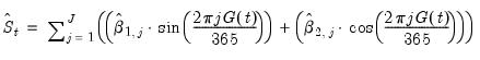 | (11.41) |
Where

denotes the exogenous terms in an ARIMA, and

is a indicator function denoting the day of the year,
i.e., cycles through

. The optimal number of trigonometric terms,

, is determine by information criteria. Note that this approximation assumes that there are exactly 365 days in a year, which requires special handling of leap years.
The order of the ARIMA model can also be determined by information criteria.
The full set of steps in Stage 2 are:
a. Remove all February 29 (leap year) observations from the DoW adjusted data produced in Stage 1.
b. Determine the optimal order of an ARIMA model using information criteria on the data created in step a), with an initial large set of trigonometric terms and any user-specified holiday, calendar or other variables as exogenous variables.
c. Determine the optimal number of trigonometric terms using information criteria based on an ARIMA model with fixed order, as determined in step b).
d. Having determined the optimal ARIMA order and number of trigonometric terms, detect outliers in the ARIMA process using the time-series outlier detection method of Chen and Liu (1993) (see below for details).
e. Estimate a final ARIMA model including effects for the detected outliers in step d) and estimate fitted values to produce a series with calendar and holiday effects removed.
f. If forecasting is required, forecast from the ARIMA model over the forecasting period.
Stage 3: Day-of-the-month adjustment
This stage takes the final data from Stage 2 and performs an STL decomposition with a periodicity of 31 to adjust for the DoM effect. This process requires that every month has exactly 31 days, and so for months with fewer than 31 days, interpolated values are inserted to extend the month to 31. The steps in Stage 3 are then:
a. Expand the adjusted data from Stage 2 so that every month has 31 days.
b. Interpolate, with a cubic spline, the inserted observations in step a).
c. Perform STL with a 31 periodicity to produce DoM adjusted data.
d. Remove the inserted observations from step a).
Stage 4: Day-of-the-year adjustment
The final seasonal adjustment performs an STL decomposition on the adjusted data from Stage 3 with a periodicity of 365 to adjust for the DoY effect.
Stage 5: Combining and forecasting
The final stage brings together the results from the previous stages and performs any forecasting. The steps in this stage are:
a. Re-insert observations for February 29, and use a cubic spline to interpolate the adjusted values from Stage 4.
b. Any holiday or event/calendar effects removed in Stage 2 are added back into the adjusted data. This produces the final seasonally adjusted (and forecasted data).
c. The final trend estimate is produced by LOESS estimation of the final adjusted data against a simple time trend.
d. The in-sample final seasonal factors are computed as the original data minus the adjusted data.
e. To produce forecasts of the seasonal factors, a forecast of the original data is required. This is computed from the ARIMA forecast in Stage 2(f), adjusted to add back the holiday/calendar effects, and the day-of-the-week seasonal factors (which are themselves forecasted using exponential smoothing, or by extending the last week of calculated seasonal factors repeated throughout the forecast).
f. Individual DoW, DoM and DoY trends and factors can be retrieved from the corresponding STL decompositions.
Outlier Detection
Stage 2 includes automatic outlier detection and correction in the ARIMA model based upon the method given in Chen and Liu (1993). In this paper, four different types of outlier effects are identified: Innovational Outlier (IO), Additive Outlier (AO), Level Shift (LS), and Temporary Change (TC).
For precise details of the procedure, we refer the reader to the original article, however as a short outline, the procedure follows these steps:
a. Calculate residuals from an initial ARIMA estimation.
b. At each time period of the estimation sample, calculate standardized statistics for each type of outlier effect.
c. If the maximum value of the statistics is greater than some critical value (cvalue), remove the effect of that outlier from the residuals, and then re-calculate the statistics in step b) using the adjusted residuals.
d. Iterate through step c) until no more outlier effects are detected at the critical value.
e. Re-estimate the ARIMA model, including outlier effects for the types and dates identified in step d) then return to step b).
f. Iterate through step e) until no new outliers are detected.
5-Day Adjustment
The original DSA algorithm is designed to handle data that are reported seven days (D7) a week. However much economic data is only reported for five days (D5) of the week, with no data available on weekends. Indeed, the application of DSA in Ollech (2021) uses five day data, and expands out the data to seven day by repeating the Friday value for Saturday and Sunday before performing DSA.
The implementation of DSA in EViews offers three alternatives for handling D5 data:
• Extend the D5 data to be D7 and use the Friday value as the value for Saturday/Sunday (as per Ollech (2021)).
• Extend the D5 data to be D7 using interpolation between Friday and Monday to fill in Saturday/Sunday values.
• Perform DSA on the D5 data itself where the daily STL has a periodicity of 5, the monthly STL has a periodicity of 23 and the yearly STL is 262. For months/years with fewer than 23/262 observations, insert observations and interpolate the missing values.
Performing Daily Seasonal Adjustment in EViews
To perform DSA seasonal adjustment in EViews, open the series and select EViews will then open a tree-structured DSA dialog to allow you to set the options for the DSA procedure:
The branches of the tree, on the left, allow you to specify the , the model, and the three STL components. Click on the node name in the left to select the node.
Basic Options
Within the Basic Options node:
• You may use the edit field to specify the end of the forecast period. The start of the forecast period will be the first observation after the current workfile sample.
If this field is blank, EViews will perform seasonal adjustment of the series over the current workfile sample, and will not forecast beyond the sample.
If the field is filled the options will be enabled, which specify how the day of the week factor should be forecasted (using either exponential smoothing, or simply extending the last week of data).
• The Output series names edit field may be used to specify the names of the output series from the procedure. If this edit field is left blank, EViews will not output the respective series.
If you workfile is structured as Daily 5-day week, the s dropdown can be used to specify how EViews will treat weekends.
• Selecting will perform DSA seasonal adjustment as though there are 262 days in each year and 23 days in each month (using interpolation to create observations for years/months with fewer days).
• Selecting either or will convert the data to a Daily 7-day week format, and fill-in the weekend values using either the value from the previous Friday, or will interpolate between the Friday and the following Monday value.
ARIMA
The node offers options for the ARIMA model estimated in Stage 2. The options are provided in separate dialog nodes: , , .
ARIMA Specification
The node controls the specification of the estimated ARIMA model:
The radio button allows you to choose between whether to tell EViews to use n to determine the appropriate order of the ARIMA model, or whether to use the with user-specified order.
• The , and dropdown menus specify the maximum orders to test if performing automatic selection, or the specified order if a fixed model is selected.
• When performing automatic selection, the dropdown allows you to specify the information criteria used to determine the most appropriate ARIMA number of trigonometric terms.
ARIMA Variables
The variables node is used to specify exogenous regressors used in the ARIMA estimation.
• The
Trig. seasonal terms section selects the number of trigonometric seasonal dummies to include in the ARIMA estimation, as defined in
Equation (11.41). You may select whether to determine automatically the number of terms using an information criterion, or you can fix the number at a specified value. Note the criterion employed for selecting the number of seasonal terms is specified in the tab (
“ARIMA Specification”).
• The box is used to enter any additional regressors you wish to include in the ARIMA estimation. Typically, variables modeling holiday patterns are used within the ARIMA estimation, and the built-in EViews function @holiday can be used to create sophisticated holiday variables.
ARIMA Outliers
Options for automatic detection of outliers in the ARIMA model can be set on the node.
The check boxes select which types of outlier to detect and model in the ARIMA, whereas the edit fields specify the parameters used during the detection process. The field specifies the critical value used to determine whether an observation contains an outlier, is used in the specification of a outlier, and the two iterations fields are used to specify the maximum number of iterations of the inner and outlier loops of the procedure.
Seasonal Adjustment
The three nodes specify options for the , , and STL decompositions. The dialog for all three types is the same:
The (or equivalent for the other month or year nodes) specifies whether to include seasonal adjustment at this periodicity. The , , and sections specify options for the STL procedure, see the STL section of UG1 for details.
The section allows you to save the outputs of the individual STL procedures as separate series. Select the desired output and then enter a name for the output series.
Example
As an example of using daily seasonal adjustment, we will work with a time-series containing daily electricity demand data for England and Wales between 2005 and 2014. The data are contained in the workfile “Elecdmd.wf1”, which contains the single series ELECDMD. The workfile extends until the end of 2015, leaving 20 months of NAs within the ELECDMD series.
Viewing a graph of this series, we can see that there are strong seasonal patterns to these data:
Not only does there appear to be a monthly pattern to electricity demand (with higher demand in the winter, as electricity is used for heating), but, if we use the slider on the bottom of the window to zoom in on a few months of data, we can see there is also a day of the week pattern:
We will use the DSA tools to remove both the seasonal and the weekly patterns. We begin by re-setting the workfile sample to begin and the workfile start and end on April 30, 2014 by issuing the command (assuming “Month/Day/Year” data handling):
smpl @first 04/30/2014
Next we open the ELECDMD series and click on to open the DSA dialog. EViews will specify a forecast end point of December 31, 2015, which is the last date in our workfile. We keep this and the remaining options in the dialog at their default values. Click to perform the adjustment.
Further, the output from the DSA will be displayed in a spool. The output is lengthy, containing detailed information on each part of the adjustment process.
For example, the displays a Trend-Seasonal-Adjusted graph for the Day-of-Week seasonal adjustment,
while the node displays a graph of the ARMA selection criterion,
and the Outliers and ARIMA Estimates show information on the outlier identification process, and the estimated ARIMA process:
Lastly, the output series will be saved in the workfile, in the case, in the series ELECDMADJ. The series will contain the DSA adjusted data, which when plotted against the original ELECDMD for the whole sample shows the effect of removing the monthly seasonality,
and when looking at a smaller time-frame, the effects of removing within-week seasonality
STL Decomposition
STL decomposition is a seasonal adjustment method that decomposes a series into seasonal, trend and remainder components using a filtering algorithm based upon LOESS regressions. Introduced by Cleveland, Cleveland, McRae and Terpenning (Cleveland henceforth) in their 1990 paper, STL has two main advantages over other seasonal adjustment methods; it works on any frequency of data, and can be calculated on time series data with irregular patterns and missing values.
STL assumes an additive relationship between the seasonal, trend and remainder components:
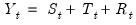 | (11.42) |
The calculation of each component involves a double recursive procedure. Specifically, the algorithm is composed of inner and outer loops with the following specification:
The Inner Loop
Let k denote the iteration parameter, running from 1 to N. np denotes the number of periods per cycle (e.g. 12 for monthly data), N the number of years. The total number of observations is then N*np (assuming we start and end at same point in cycle). Let RW denote a passed in weighting series.
1. Create a series of detrended values,
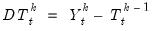
, using previous Trend estimate,

.
2. Split the detrended series into np sub-series each of length NI. E.g. create a series containing just January values, another containing just February values. For each of these sub-series, perform LOESS to create smoothed values. In computation of the LOESS weights, the weights are further weighted by RW.
• Smoothed values are also created for any missing values, and for 1 cycle (year) prior to and after the data sample. For example, if we have monthly data from 2000 to 2010, then we first create smoothed values for Jan 1999, Jan 2000, Jan 2001, …, Jan 2010, Jan 2011. Then smoothed values for Feb 1999, Feb 2000, …, Feb 2010, Feb 2011, and so on. This results in having 2 extra smoothed observations per sub-series. Or (2+
N)*
np in total. The results are stored in series

.
3. For each smoothed sub-series, perform 3 moving average calculations, recursively. These moving average calculations result in the loss of 2 observations per sub-series, but since we created an extra 2 observations in Step 2, we end up with the correct number of observations. The thrice MA’d series are then smoothed with another LOESS smoothing and stored in series

.
4. Calculate an estimate of the seasonal values,
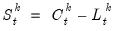
.
5. Deseasonalize,
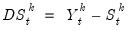
.
6. Smooth

with LOESS smoothing to compute

. In computation of the LOESS weights, the weights are further weighted by
RW. The initial trend estimate,

, is set equal to zero.
The Outer Loop
After the iterations of the inner loop are completed, we are left with an estimate of the trend,

, and of the seasonal component,

. We can estimate the remainder component as:
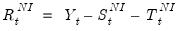 | (11.43) |
To correct for outliers, the remainder series is used to calculate robustness weights. Let
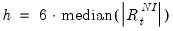
, then
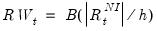
, where
B is the bisquare function:
 | (11.44) |
RW is then fed in to the next set of iterations of the inner loop. The initial set of RW are set at 1.
LOESS Estimation
The heart of the STL procedure is the heavy use of LOESS estimation to create smoothed values of data. STL uses LOESS with a tri-cube function with either a locally linear or locally quadratic polynomial. To smooth the time series
A, we first create a trend variable
T, running from 1 to
T (number of observations in
A). We smooth each value in
A one at a time. Each value of
A,

, has a corresponding trend value,

. To calculate the smoothed value of

we take the
k observations of
A and
T around

to form new smaller time series,

and

.
Weights are then calculated as:
Where W is the tri-cube function:
And

is the furthest distance of

from the values in

:
The weights may then be used to either calculate a weighted average of the

as an estimate of

(if using a locally-linear polynomial) or to perform weighted least squares of

against

and use the coefficients to produce a fitted value of

(if using a locally quadratic polynomial).
When estimating using the LOESS, the size of the window, k must be decided. Cleveland recommend a seasonal smoothing (Step 2) window of at least 7. Larger values increase the smoothness of the seasonal component.
Setting the seasonal smoothing window larger than the sample size will guarantee that the seasonal components are constant across cycles (e.g. the January value is the same each year, the February value is the same each year, and so on). Shorter values can lead to large variations in the seasonal components across years.
Selecting the correct smoothing windows size can be difficult. Cleveland suggest a graphical diagnostic tool, termed the seasonal-diagnostic plot, which graphs the relationship between the demeaned seasonal component and the demeaned seasonal component plus the remainder component for each period. Smooth seasonal lines imply a reasonable choice of seasonal window.
For the trend smoothing (Step 6), Cleveland recommend a value between 1.5np and 2np. For the filter window (Step 3), the lowest integer greater than np is recommended.
Missing Values
The LOESS smoothing technique used at to produce the seasonal and trend components of the procedure is able to produce values even when the underlying data is missing. The procedure is only unable to calculate a smoothed value if there are not enough observations in the LOESS window with valid data. A locally linear polynomial requires at least one valid observation inside the window, and the locally quadratic polynomial requires at least two.
STL Decomposition in EViews
To perform STL Decomposition of a series in EViews click on to bring up the dialog:
The box allows you to specify the periodicity of your data - number of periods per cycle. This will usually be set to the number of periods per year for the frequency of your data, for example monthly data has a periodicity of 12. This number must be set to a positive integer.
Weekly and daily data are problematic since there is not an integer number of weeks or days in a year. EViews can still compute STL Decomposition in these cases by expanding each year of data so that it has a full set of periods. For example, for weekly data each year is expanded so that it has exactly 53 weeks. Any years that actually have 52 weeks are expanded to have an extra observation (filled with an NA). Similarly, daily data is expanded to have 366 observations per year. To instruct EViews to perform this expansion on weekly data, enter rather than an integer number as the periodicity. For daily data, enter .
If your workfile is an irregular dated workfile (i.e. some observations are missing from the workfile), and has a frequency of either semi-annual, quarterly, monthly, weekly or daily, and you set the periodicity to be one year (e.g. 12 for monthly data, 2 for semi-annual data, for daily data), EViews will adjust the STL procedure so that the dates in each year continue to line up, even with the missing observations.
The area specifies the polynomial degree of the LOESS estimations. The seasonal polynomial degree corresponds to the that used during Step 2 of the inner loop of the STL procedure. The trend polynomial degree is used during Step 6, and the filter polynomial is used during Step 3.
Similarly, the specifies the size of the window, k, used during the LOESS estimations of Step 2 (seasonal), Step 6 (trend) and Step 3 (filter). These smoothing window lengths must be odd integers.
The area can be used to specify the names of the seasonal and trend series that will be created as part of the STL procedure. You may also optionally provide a forecast length. If specified, EViews will take the average of the last three cycle’s seasonal values as a forecast of the seasonal component, and will linearly extrapolate from the last three cycle’s trend values as a forecast of the trend component. The checkbox instructs EViews to display the seasonal diagnostics plot recommended by Cleveland to determine the correct seasonal window length.
specifies the number of times the inner loop and outer loop are computed. If you believe your data has a small number of outliers, the outer loop iterations can be set to a small number such as 1 or 2. Cleveland’s original paper suggests that the inner loop converges quickly, so a low number can also be used for the number of inner loop iterations.
The box allows you to specify the sample used to perform the decomposition. Note that unlike the other seasonal adjustment methods in EViews, STL Decomposition does not require a continuous sample with no missing values.
Clicking on the STL dialog will produce the results of the decomposition. EViews will display a graph of the original data, along with the seasonal, trend and remainder components, and if requested, the seasonal diagnostics plot.
Examples
As an example of using STL decomposition, we will replicate one of the studies performed in the original Cleveland paper using monthly averages of measurements of atmospheric C02 by the Scripps Institute of Oceanography between 1959 and 1987 (the data are in the CO2.wf1 workfile). A quick graph of the original data shows it exhibits strong seasonality with a clear upward trend:
We will use the STL procedure to decompose this time series into seasonal and trend components. We click on to open the dialog:
Following Cleveland’s example, we set the seasonal polynomial degree to , and the other two to . We use a seasonal smoothing window of , a trend window of and a filter of . Cleveland use short iteration loops, setting the inner loop at just iterations, and the outer loop at . We choose to produce the seasonal diagnostic plot. Clicking produces the two sets of output graphs:
The first set of graphs shows the original data, labeled CO2, the decomposed trend component, the seasonal component and the remainder. The trend is a near straight upward trending line, and the seasonal component, although allowed to change through time, is consistent with high values approaching 3 every May and low values passing -3 every October. The relatively flat lines in each of the Seasonal Diagnostics panels indicate that the choice of 35 as the seasonal window was appropriate.
As a second example we will decompose a series of weekly electricity demand in England and Wales between April 2005 and April 2013. The data is missing values in April 2005 and June 2005. The data are contained in the workfile elecdmd_weekly.wf1, which has a range of April 2005 until April 2015 (i.e. two extra years of observations are included in the workfile). A graph of the data displays clear seasonal patterns:
Note the gaps in the line corresponding to the missing values in early 2005.
We will use the STL procedure to decompose this time series into seasonal and trend components. We click on to open the dialog:
We will leave all settings at their default value, other than changing the length of the seasonal smoother to . Note that since we have weekly data, the Periodicity box is pre-filled in with the value “w”. Our data runs from 2005 until 2013. Over that time period each year has 52 weeks apart from 2010, which has 53 weeks.
Also note that we have selected to forecast the seasonal and trend components beyond the end of the data, by entering “104” as the number of forecast periods (two years).
Clicking produces a graph of the estimated seasonal, trend and remainder components:
The trend components is less linear than our previous example, with a clear downward path between 2006 and 2011, followed by an upward path.
Moving Average Methods
Ratio to moving average—multiplicative
The algorithm works as follows. Denote the series to be filtered by

.
1. First compute the centered moving average of

as:
 | (11.45) |
2. Take the ratio

.
3. Compute the seasonal indices. For monthly series, the seasonal index

for month

is the average of

using observations only for month

. For quarterly series, the seasonal index

for quarter

is the average of

using observations only for quarter

.
4. We then adjust the seasonal indices so that they multiply to one. This is done by computing the seasonal factors as the ratio of the seasonal index to the geometric mean of the indices:
 | (11.46) |
5. These

are the reported
scaling factors in the series window and are saved as series if you provide a name in the field box. The interpretation is that the series

is

percent higher in period

relative to the adjusted series.
6. The seasonally adjusted series is obtained by dividing

by the seasonal factors

.
Difference from moving average—additive
Suppose that we wish to filter

.
2. Take the difference

.
3. Compute the seasonal indices. For monthly series, the seasonal index

for month

is the average of

using observations only for month

. For quarterly series, the seasonal index

for quarter

is the average of

using observations only for quarter

.
4. We then adjust the seasonal indices so that they add up to zero. This is done by setting

where

is the average of all seasonal indices. These

are the reported
scaling factors. The interpretation is that the series

is

higher in period

relative to the adjusted series.
5. The seasonally adjusted series is obtained by subtracting the seasonal factors

from

.
The main difference between X11 and the moving average methods is that the seasonal factors may change from year to year in X11. The seasonal factors are assumed to be constant for the moving average method.
Census X11 (Historical)
While available in earlier versions of EViews, the X11 programs, as provided by the Census, do not run on 64-bit operating systems and are no longer supported.
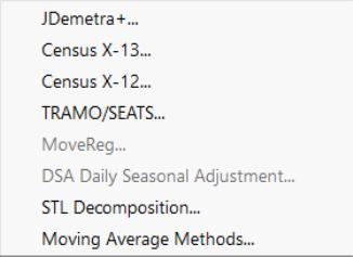
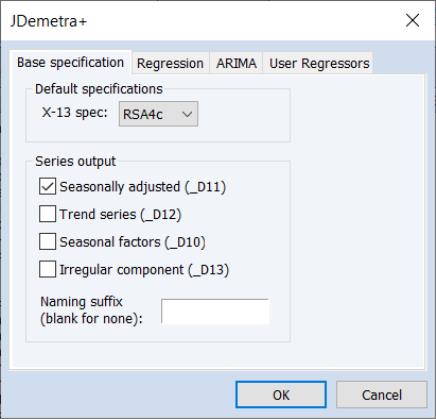
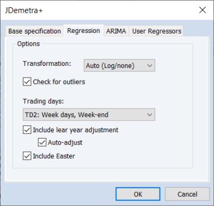
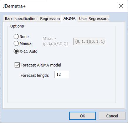
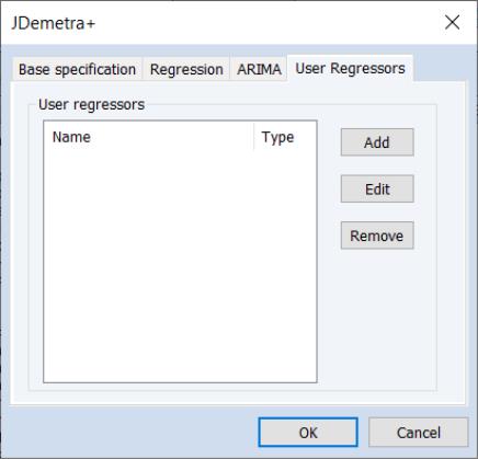
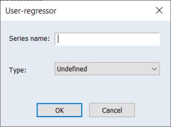
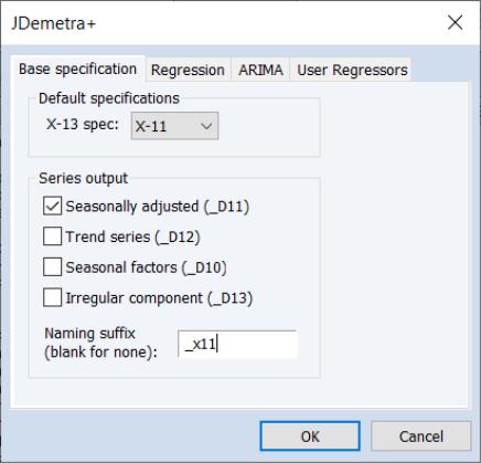
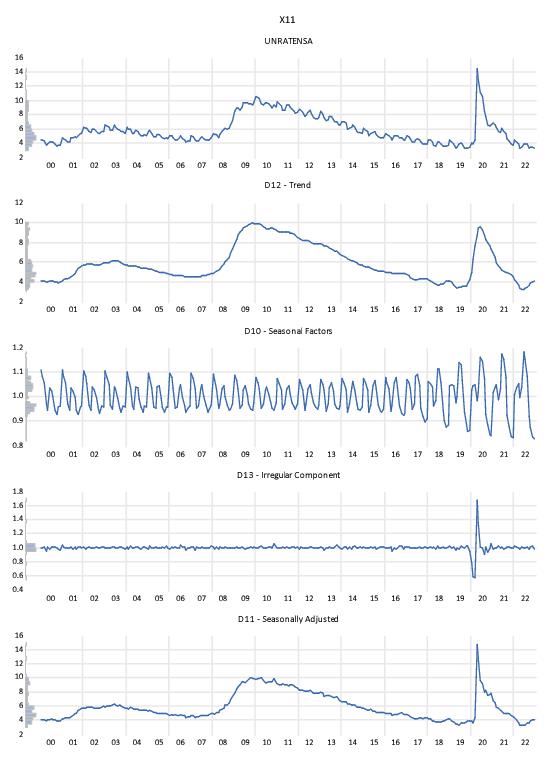
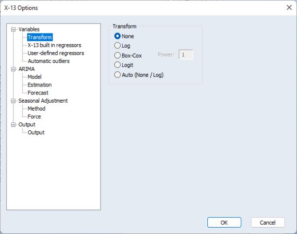
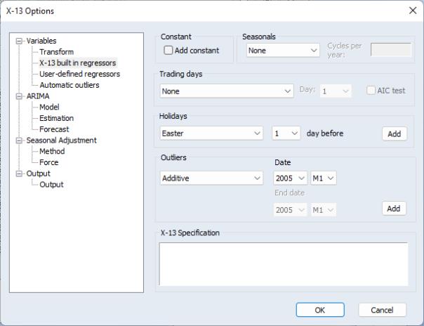
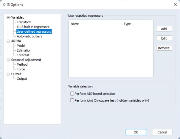
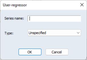
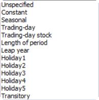
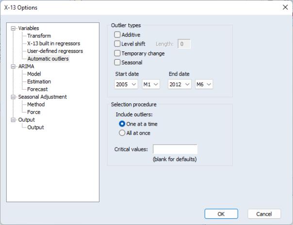
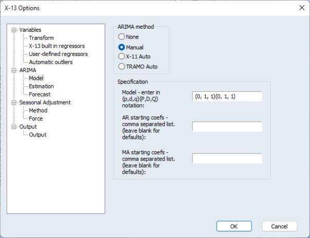
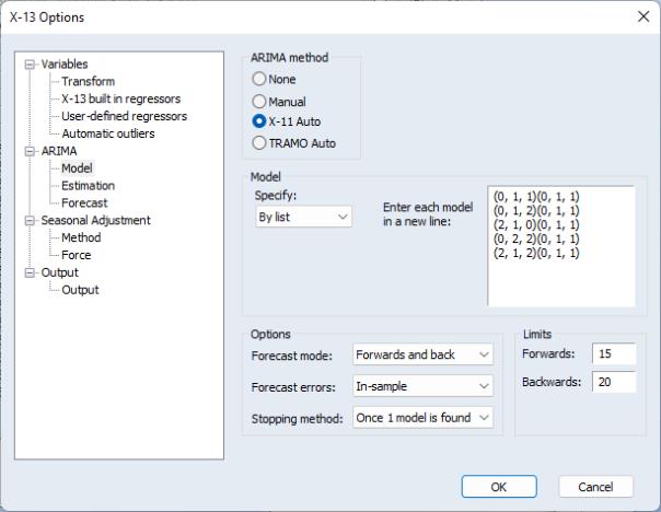
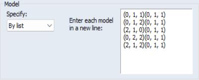
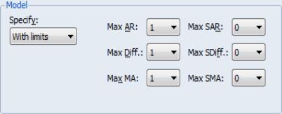
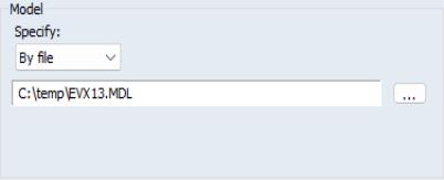
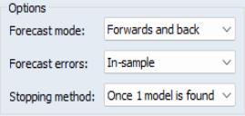
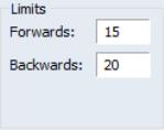
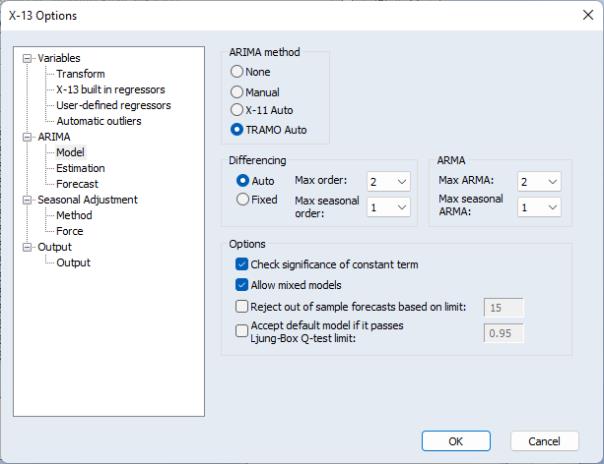
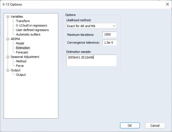
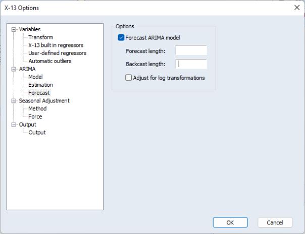
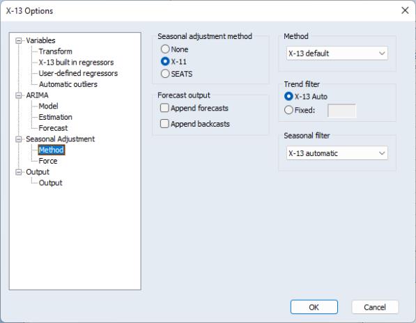
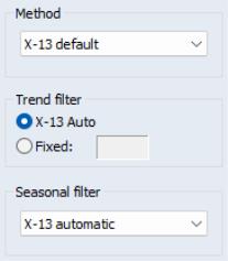
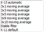
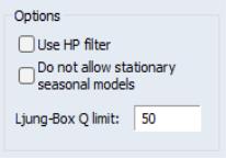
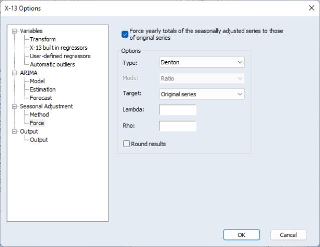
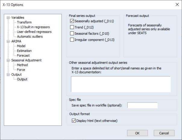
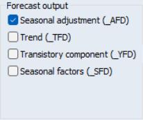
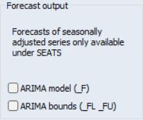
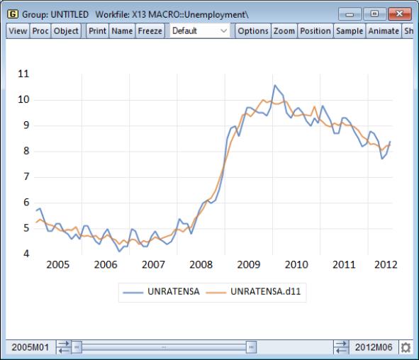
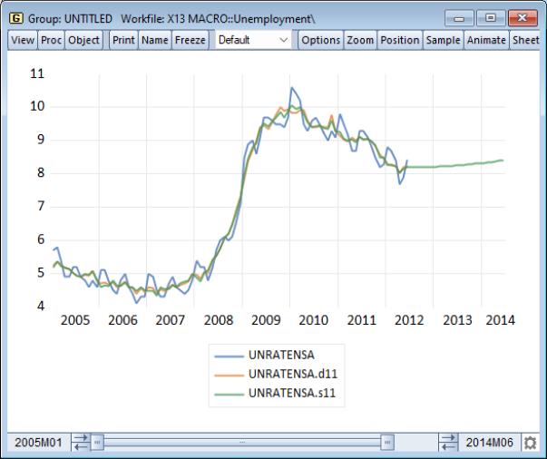
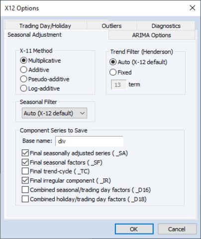
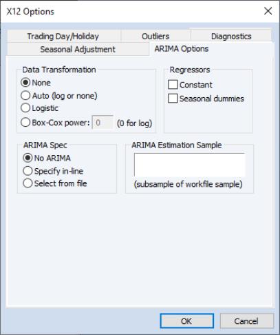
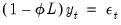
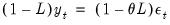
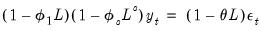
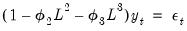
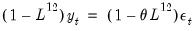
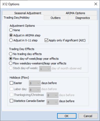
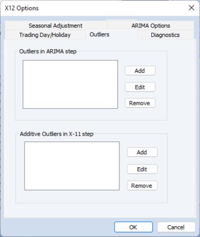
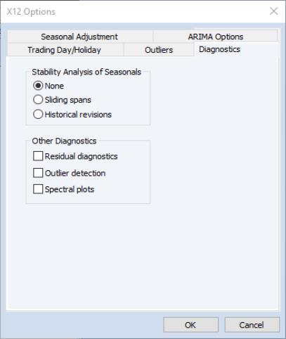
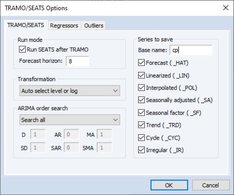
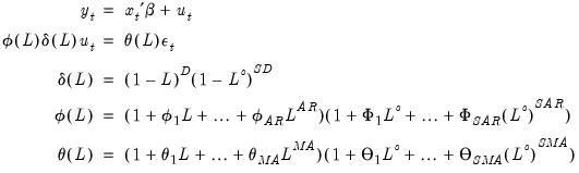
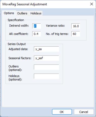
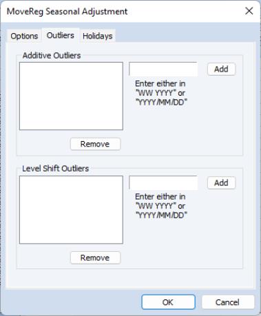
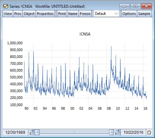
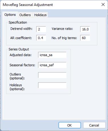
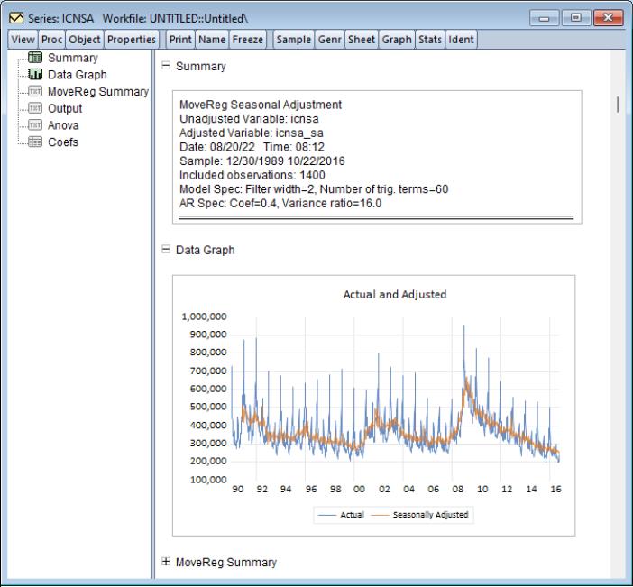
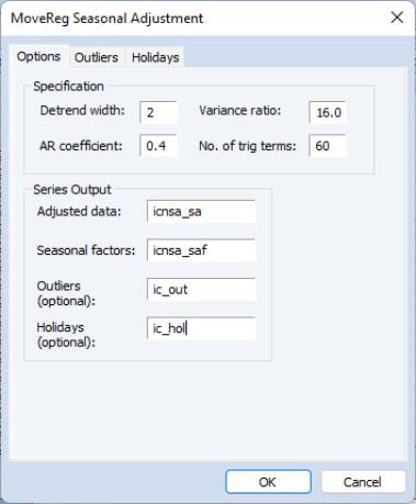
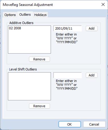
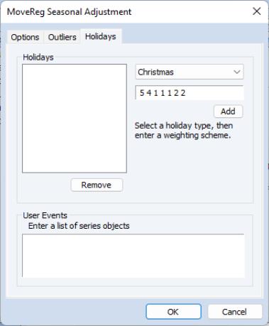
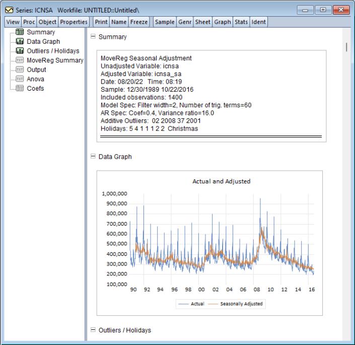
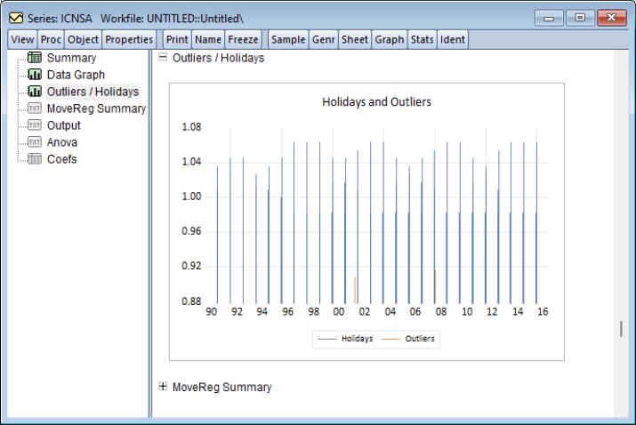
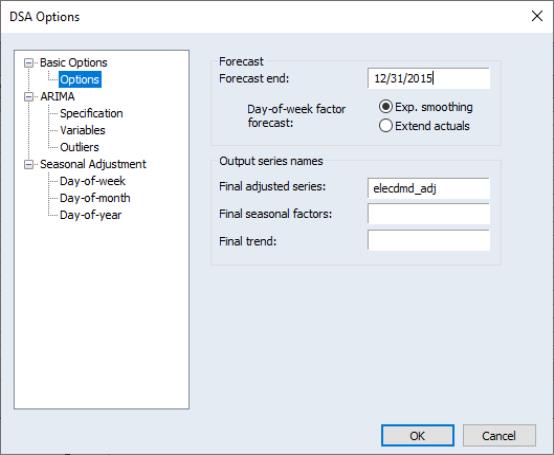
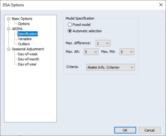
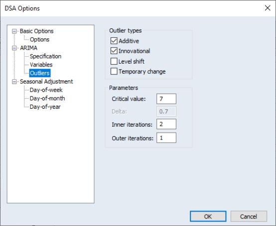
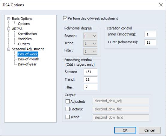
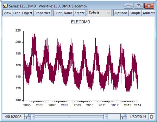
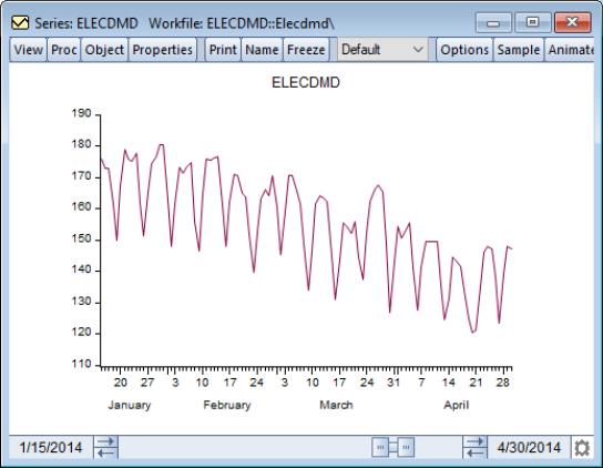
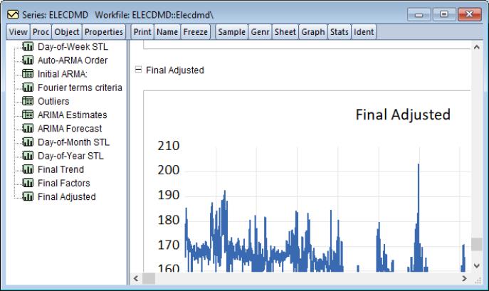
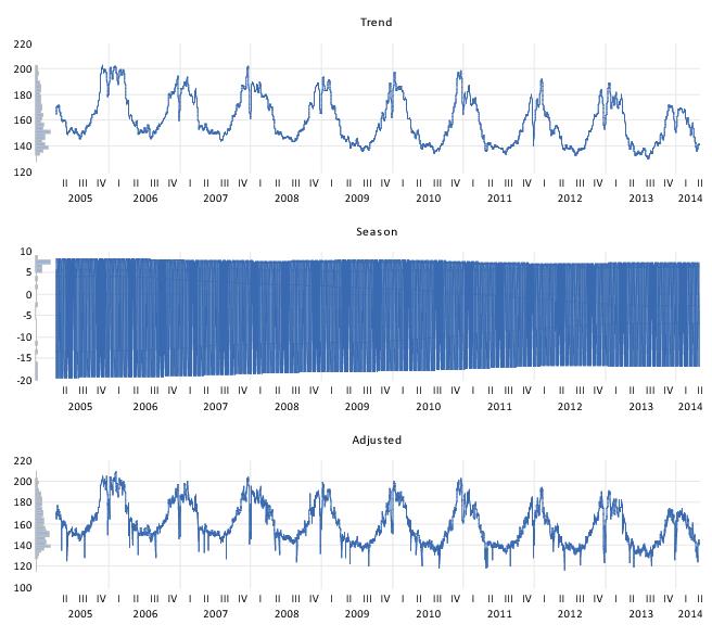
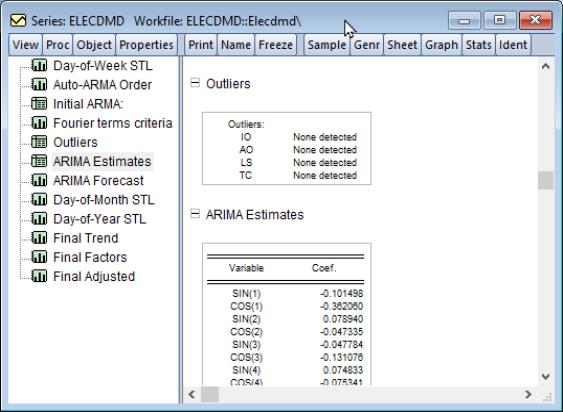
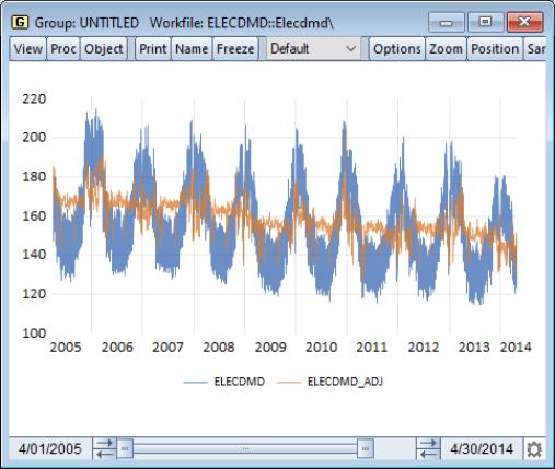
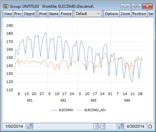
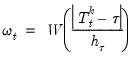
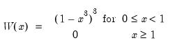
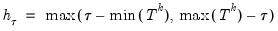
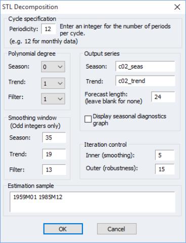
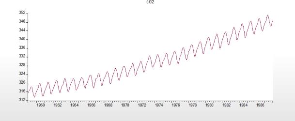
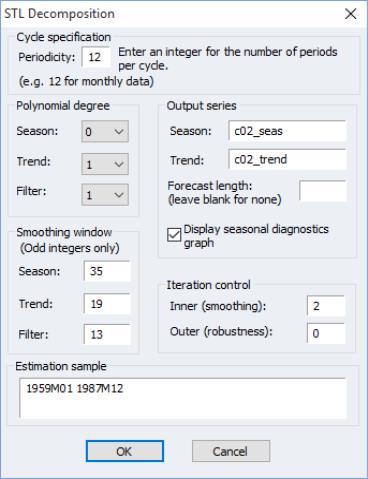
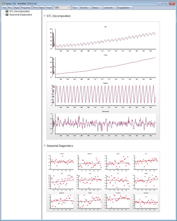
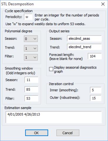
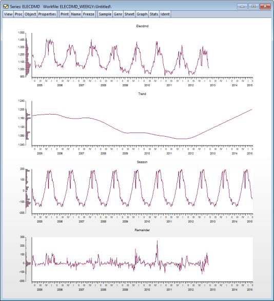
 as in
as in