Function Reference: T
@tan Tangent of argument specified in radians.
@tdist Tail probabilities of the Student’s
t distribution.
@temppath Directory path for EViews temporary files.
@theil Theil inequality coefficient (difference) between series.
@time Current time as a string.
@toc Elapsed time (since timer reset) in seconds.
@trace Computes the trace of a square matrix or sym.
@trendc Trend series using calendar dates.
@trendcoef Trend coefficient from detrending a series.
@trigamma Second derivative of the natural log gamma function.
@trim Trim left and right whitespace from string.
@tz Convert time in source time zone to destination time.
@tzlist Available time zone specifications.
Table and sheet names in a foreign file.
Syntax: @tablenames("str")
str: string
Return: string
Returns a space delimited string containing the names of the table names of a foreign file. The name (and path) of the foreign file should be specified in str, enclosed in quotes.
For an Excel file, the names of the Excel sheets will be returned.
Tangent of argument specified in radians.
Compute the tangent of x (specified in radians).
Syntax: @atan(x)
x: number
Return: number
Examples
= @tan((5/4)*@pi)
returns 1.
Cross-references
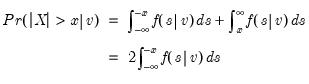
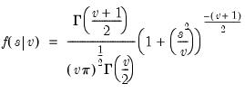
Tail probabilities of the Student’s

distribution.
Syntax: @tdist(x, v)
x: number
v: number,

Return: number
Probability that a t-statistic
with  degrees of freedom exceeds
  in absolute value (two-sided p
-value
). due to symmetry, where
Examples
= @tdist(-12.71, 1)
returns 0.04998....
Cross-references
Directory path for the EViews temporary files.
Syntax: @temppath
Return: string
Returns a string containing the directory path for the EViews temporary files as specified in the global options menu
Examples
If your currently executing copy of EViews puts temporary files in “D:\EVIEWS”, then:
%y = @temppath
assigns a string of the form “D:\EVIEWS”.
Cross-references
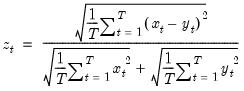
Theil inequality coefficient (difference) between series.
Computes the Theil inequality coefficient of x and y.
Syntax: @theil(x, y, [s])
x: series
y: series
s: (optional) sample string or object
Return: number
The Theil inequality coefficient is given by the root mean square error divided by the sum of the square roots of the squared x and squared y means).
Examples
Let yf denote in-sample forecasts for the series y. Then
= @theil(yf, y)
returns the Theil inequality coefficient between the series y and its forecast.
Cross-references
Current time as a string.
Syntax: @time
Return: string
Returns a string containing the current time in “hh:mm” format.
Examples
%y = @time
assigns a string of the form “15:35”.
Cross-references
Elapsed time (since timer reset) in seconds
Syntax: @toc
Return: integer
Compute elapsed time (since timer reset) in seconds.
Examples
tic
[some commands]
!elapsed = @toc
resets the timer, executes commands, and saves the elapsed time in the control variable !ELAPSED.
Cross-references
Computes the trace of a square matrix or sym.
Syntax: @trace(m)
m: matrix, sym
Return: scalar
Returns the trace (the sum of the diagonal elements) of a square matrix or sym, m.
Examples
matrix m1 = @mnrnd(10, 10)
scalar sc1 = @trace(m1)
scalar sc2 = @sum(@getmaindiagonal(m1))
generate a random matrix, and then compute the trace directly and indirectly.
Similarly,
matrix s1 = @inner(@mnrnd(100, 20))
scalar sc1a = @trace(s1)
scalar sc2a = @sum(@getmaindiagonal(s1))
generate a random sym, and then compute the trace in two ways.
Cross-references
Transpose of a matrix object.
Syntax: @transpose(m)
m: matrix, vector, rowvector, sym
Return: matrix, rowvector, vector, sym
The result is a matrix object with the number of rows and columns and the element indices reversed from the original matrix. This function is an identity function for a sym, since a sym by definition is equal to its transpose.
Examples
matrix m1 = @mnrnd(5, 7)
matrix m1t = @transpose(m1)
creates a

matrix M1 filled with normal random variables, and the

matrix transpose.
vector v1 = @mnrnd(10)
matrix m2 = v1 * @transpose(v1)
matrix m3 = @outer(v1, v1)
creates the 10-element vector V1 and forms its

outer product matrix in two ways.
Note that the transpose of matrix objects may also be obtained using the “@t” object data member function, as in
matrix m4 = v1 * v1.@t
Cross-references
Trend.
Syntax: @trend([d])
d: (optional) date or observation
Return: series
Returns a time trend that increases by one for each observation in the workfile.
The optional date or observation d may be provided to indicate the starting point (with a 0 value) for the trend. If d omitted, the starting point is assumed to be the earliest date in the workfile.
This function is panel aware. In this context, trend values are defined sequentially across the entire set of available cross-section dates, and then matched to the individual cross-section dates. If there is a specific date that is missing in one cross-section, but is present in another, there will be a gap (non-sequential values) in the trend in the former. Thus, the panel trend may be thought of as a calendar trend that uses the calendar defined by dates observed in the workfile.
For a trend function that uses calendar dates, use
@trendc. For a simple panel trend in which values begin at 1 and sequentially increase by 1, you may use the
@obsid function.
Examples
series t = @trend
creates a trend series starting at 0 in the first workfile observation.
series t90q1 = @trend("1990q1")
creates a trend series based at 0 in 1990q1.
Cross-references
Trend with break.
Syntax: @trendbr([d])
d: (optional) date or observation
Return: series
Returns a breaking time trend that is zero for each observation prior to and at the break point, and increases by one for each observation following the break.
The optional date or observation d may be provided to indicate the break/starting point for the trend. If d omitted, the break point is assumed to be the first observation, and the function produces a simple trend.
This function is panel aware. In this context, trend values are defined sequentially across the entire set of available cross-section dates, and then matched to the individual cross-section dates. If there is a specific date that is missing in one cross-section, but is present in another, there will be a gap (non-sequential values) in the trend in the former. Thus, the panel trend may be thought of as a calendar trend that uses the calendar defined by dates observed in the workfile.
To obtain a simple panel trend in which values begin at 1 and sequentially increase by 1, you may use the
@obsid function.
Examples
series tbr90q1 = @trendbr("1990q1")
creates a trend series based at 0 in 1990q1. Observations before 1990q1 will be set to 0; observations after 1990q1 will sequentially increase by 1.
Cross-references
Calendar trend.
Syntax: @trendc([d])
d: (optional) date or observation
Return: series
Returns a calendar time trend that increases by the number of calendar periods between successive observations.
The optional date or observation d may be provided to indicate the starting point (with a 0 value) for the trend. If d omitted, the starting point is assumed to be the earliest observation in the workfile.
• In a regular frequency workfile, @trend and @trendc both return a simple trend that increases by one for each observation of the workfile.
• In an irregular workfile, @trend provides an observation-based trend as before, but @trendc now returns a calendar trend that increases based on the number of calendar periods between adjacent observations. For example, in a daily irregular file where a Thursday has been omitted because it was a holiday, the @trendc value would increase by two between the Wednesday before and the Friday after the holiday, while @trend will increase by only one.
This function is panel aware. For a panel trend function that uses only the observed dates, use
@trend. For a simple panel trend in which values begin at 1 and sequentially increase by 1, you may use the
@obsid function.
Examples
series t = @trend
creates a calendar trend series starting at 0 in the first workfile observation.
series t90q1 = @trend("1990q1")
creates a calendar trend series based at 0 in 1990q1.
Cross-references
Trend coefficient from detrending regression.
Computes the trend coefficient (or coefficients for panel data) of an OLS regression versus a constant and an implicit time trend.
Syntax: @trendcoef(x[, s])
x: series, vector, matrix
s: (optional) sample string or object when x is a series and assigning to series
Return: number
Returns the trend coefficient of an OLS regression on matrix or vector m versus a constant and an implicit time trend, as in @detrend.
When applied to a matrix, the matrix elements are arranged in vectorization order and then paired with the implicit time trend.
This function is panel aware.
For series calculations, EViews will use the current or specified workfile sample.
Examples
series y = 2 + 3 * @trend + @nrnd
= @trendcoef(y)
The first line generates the series y using a simple linear regression model, where the sole regressor is a time trend, the intercept is 2, and the slope coefficient is 3. The second line returns the OLS estimate of the slope coefficient, and is approximately 3 in large samples.
The following commands begin by creating a workfile, generating a random series, and then converting to a vector so that we can compute identical results using the series and the vector.
workfile u 100
series y = nrnd
vector yv = @convert(y)
The trend regression trend coefficient estimate is given by
scalar tr1 = @trendcoef(yv)
Alternately, the trend regression results may be obtained using the vector YV using the @regress command on the augmented data matrix:
matrix vcoefs = @regress(@hcat(yv, @ones(yv.@rows), @range(0, yv.@rows-1)))
The first column of VCOEFS contains the intercept and trend coefficient, so
scalar tr2 = vcoefs(2)
is the trend coefficient.
Estimates may also be obtained using the series and an equation object
equation eq1.ls y c @trend
scalar tr3 = eq1.c(2)
Cross-references
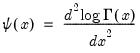
Second derivative of the natural log gamma function.
Syntax: @trigamma(x)
x: number
Return: number
for  .
. Examples
= @trigamma(0.5)
returns 4.93480... (equivalent to

).
Cross-references
Trim left and right whitespace from string.
Syntax: @trim(str)
str: string, alpha, svector
Return: string, alpha, svector
Returns the string str with spaces trimmed from the left and the right.
Examples
@ltrim(" I doubt that I did it. ")
returns “I doubt that I did it.” after trimming off spaces from both ends.
If ALPHA1 is an alpha series,
alpha alphaltrim = @trim(alpha1)
returns the left and right-trimmed strings in ALPHA1 for each observation in the workfile sample.
If SVEC1 is an string vector,
svector sveclen = @trim(svec1)
returns a string vector containing the left and right-trimmed elements of SVEC1.
Cross-references
See also
@ltrim and
@rtrim.
Trimmed mean.
Compute the mean after the p-percent largest and smallest values have been removed.
Syntax: @trmean(x, p[, s])
x: series, vector, matrix
p: number, series, vector, matrix
s: (optional) sample string or object when x is a series and assigning to a series
Return: number
For
x with

observations and

, define the number of trimmed end observations as
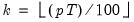
, where

is the integer floor function.
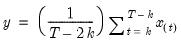
Then the trimmed mean is given by
where the order statistics

represent data for the

observations ordered from low to high,
For series calculations, EViews will use the current or specified workfile sample.
Examples
= @trmean(y, 5)
computes the 5% trimmed mean for series y.
Consider the commands
matrix m = @mrnd(10,10)
m(1,1) = 1000
scalar om = @mean(m)
scalar trm = @trmean(m,1)
The mean of M should be approximately 10.495, whereas the trimmed mean (with the largest and smallest 1% trimmed off) should be close to 0.5.
Cross-references
Convert time in source time zone to destination time.
Syntax: @tz((srctime, srctzone, destzone)
srctime: date number
srctzone: string
destzone: string
Return: date number
Converts a point in time srctime from the source time zone srctzone into the corresponding time in the destination time zone destzone.
• The
srctzone and
destzone strings can either contain raw time zone information in the format returned by
@tzspec or they can contain search text (such as a city name) found within one of the time zone descriptions returned by the function
@tzlist.
Examples
series localtime = @tz(utctime, "London", "Sydney")
converts a series containing time values in London local time into equivalent local time values in Sydney.
Cross-references
See
“Dates” and
“Event Functions” for related discussion.
See also the related time zone functions
@utc,
@localt,
@tzlist, and
@tzspec.
Available time zone specifications.
Syntax: @tzlist
Return: string
Returns a space delimited list of descriptions of all the time zones for which information is available on the current machine.
Examples
string all_specs = @tzlist
saves the list of all available time zone specifications for the current machine to the string object ALL_SPECS.
Cross-references
See
“Strings” and
“Event Functions” for related discussion.
See also the related time zone functions
@utc,
@localt,
@tz, and
@tzspec.
Time zone specification.
Syntax: @tzspec(str)
str: string
Return: string
Returns time zone information for the first time zone whose description contains the piece of text passed in as str.
tr can be a city name such as “London” or “Tokyo” or any other word from the time zone description such as “Eastern” for the U.S. Eastern Time Zone.
Time zone information specifications have the format:
standard_utc_bias [daylight_offset daylight_start_rule daylight_end_rule]
where:
• standard_utc_bias is the offset (in +/– hh:mi format) of local time from UTC when daylight time is not in effect.
• daylight_offset is the additional adjustment (in +/– hi:mi format) to the standard UTC bias when daylight time is in effect.
• daylight_start_rule is the day/time when the daylight time adjustment begins. This can be an explicit date or a date rule.
• daylight_end_rule is the day/time when the daylight time adjustment ends. This can be an explicit date or a date rule.
If there have been historical changes to the time zone rule, each era is returned beginning with an “@” symbol followed by the year in which the new rule took effect. The year may be dropped to indicate that the rule should be applied to all earlier dates.
For example, a historical description of the Pacific Time Zone (PT) description for parts of western Canada, the western United States, and western Mexico (valid from 1987 onwards) has the specification:
@2007 -08:00 +01:00 Mar2Sun 2AM to Nov1Sun 2AM
@ -08:00 +01:00 Apr1Sun 2AM to Oct-1Sun 2AM
The standard offset of the Pacific Time Zone from UTC is -8 hours. The daylight rule after 2007 has been to move clocks forward by one hour at 2AM on the second Sunday of March and move them back at 2AM on the first Sunday in November. Before 2007 the rule was to move clocks forward by one hour at 2AM on the first Sunday of April, and move them back at 2AM on the last Sunday in October.
Examples
The command
string london_spec = @tzspec("London")
assigns a text description of the London time zone specification (Greenwich Mean Time (GMT) during standard time and British Summer Time (BST) during Daylight Saving Time (DST)),
+00:00 +01:00 Mar-1Sun 1:00 to Oct-1Sun 2:00
to the string object LONDON_SPEC, while
string eastern_spec = @tzspec("Eastern")
assigns the U.S. Eastern Time Zone (ET) description
@2007 -05:00 +01:00 Mar2Sun 2:00 to Nov1Sun 2:00 @ -05:00 +01:00 Apr1Sun 2:00 to Oct-1Sun 2:00
to the string object EASTERN_SPEC.
If ALPHA1 is an alpha series, the command
alpha a1 = @tzspec(alpha1)
fills A1 with time-zone specifications associated with the spec in ALPHA1, for each observation in the workfile sample.
If AVEC1 is an svector, the commands
svector s1 = @tzspec(avec1)
creates a vector of time-zone specifications corresponding to elements of AVEC1.
Cross-references
See
“Dates” and
“Event Functions” for related discussion.
See also the related time zone functions
@utc,
@localt,
@tz, and
@tzlist.