Function Reference: C
@cagr Compound annual growth rate of series (in decimal fraction).
@capplyranks Reorder the rows of the matrix using a vector of ranks.
@cbeta Beta cumulative distribution function.
@cbinom Binomial cumulative probability function.
@cbvnorm Bivariate normal cumulative distribution function.
@cchisq Chi-square cumulative distribution function.
@ceil Smallest number greater than or equal to (with optional precision
).
@cellid Within cross-section identifier series for panel workfile observation.
@cexp Exponential cumulative distribution function.
@cextreme Extreme value (Type I-minimum) cumulative distribution function.
@cfdist F-distribution cumulative distribution function.
@cfirst First non-missing value in each column of a matrix.
@cgamma Gamma cumulative distribution function.
@cged Generalized error cumulative distribution function.
@chisq Upper tail of the Chi-square cumulative distribution function.
@chr ASCII value to string character.
@cifirst Index of the first non-missing value in each column of a matrix.
@cilast Index of the last non-missing value in each column of a matrix.
@cimax Index of the maximal value in each column of a matrix.
@cimin Index of the maximal value in each column of a matrix.
@cintercept Intercept from a trend regression performed on each column of a matrix.
@claplace Laplace cumulative distribution function.
@clast Last non-missing value in each column of the matrix.
@clogistic Logistic cumulative distribution function.
@cloglog Complimentary log-log function.
@clognorm Log normal cumulative distribution function.
@cmax Maximal value in each column of a matrix.
@cmean Mean in each column of a matrix.
@cmedian Median of each column of a matrix.
@cmin Minimal value for each column of the matrix.
@cnas Number of NA values in each column of a matrix.
@cnegbin Negative binomial cumulative probability function.
@cnorm Standard normal cumulative distribution function.
@cobs Number of non-NA values in each column of a matrix.
@colcumprod Cumulative products for each column of a matrix.
@colcumsum Cumulative sums for each column of a matrix.
@colpctiles Percentile values for each column of a matrix.
@colranks Ranks of each column of the matrix.
@colsort Sort each column of the matrix.
@colstdize Standardize each column using the sample (d.f. corrected) standard deviation.
@colstdizep Standardize each column using the population (non-d.f. corrected) standard deviation.
@columns Number of columns in matrix object or group.
@cond Condition number of square matrix or sym.
@convert Converts series or group to a vector or matrix after removing NAs.
@cor Correlation of two vectors or series, or between the columns of a matrix or series in a group.
@cos Cosine of argument specified in radians.
@cov Covariance (non-d.f.corrected) of two vectors or series, or between the columns of a matrix or series in a group.
@covp Covariance (non-d.f. corrected) of two vectors or series, or between the columns of a matrix or series in a group.
@covs Covariance (d.f. corrected) of two vectors or series, or between the columns of a matrix or series in a group.
@cpareto Pareto cumulative distribution function.
@cpoisson Poisson cumulative probability function.
@cprod Product of elements in each column of a matrix.
@crossid Cross-section identifier series for panel workfile observation.
@cstdev Sample standard deviation (d.f. corrected) of each column of a matrix.
@cstdevp Population standard deviation (non-d.f. corrected) of each column of a matrix.
@cstdevs Sample standard deviation (non-d.f. corrected) of each column of a matrix.
@csum Sum of the values in each column of a matrix.
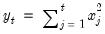
@csumsq Sum of the squared values in each column of a matrix.
@ctdist Student’s

cumulative distribution function.
@ctrendcoef Slope from a trend regression on each column of a matrix.
@ctrmean Trimmed mean of each column of a matrix.
@cumbmax Backward cumulative maximums of a series.
@cumbmean Backward cumulative means of a series.
@cumbmin Backward cumulative medians of a series.
@cumbnas Backward cumulative number of missing observations of a series.
@cumbobs Backward cumulative number of (non-missing) observations of a series.
@cumbprod Backward cumulative products of a series.
@cumbstdev Backward cumulative standard deviations (d.f. corrected) of a series.
@cumbstdevp Backward cumulative standard deviations (non-d.f. corrected) of a series.
@cumbstdevs Backward cumulative standard deviations (d.f. corrected) of a series.
@cumbsum Backward cumulative sums of a series.
@cumbsumsq Backward cumulative sums-of-squares of a series.
@cumbvar Backward cumulative variances (non-d.f. corrected) of a series.
@cumbvarp Backward cumulative variances (non-d.f. corrected) of a series.
@cumbvars Backward cumulative variances (d.f. corrected) of a series.
@cumdn Cumulative sum of negative (below threshold) changes in a series.
@cumdp Cumulative sum of positive (above threshold) changes in a series.
@cumdz Cumulative sum of zero (at threshold) changes in a series.
@cummax Cumulative maximums of a series.
@cummin Cumulative minimums of a series.
@cumnas Cumulative number of missing observations of a series.
@cumobs Cumulative number of (non-missing) observations of a series.
@cumprod Cumulative products of a series or the elements of a matrix.
@cumstdev Cumulative standard deviations (d.f. corrected) of a series.
@cumstdevp Cumulative standard deviations (non-d.f. corrected) of a series.
@cumstdevs Cumulative standard deviations (d.f. corrected) of a series.
@cumsum Cumulative sums of a series or the elements of a matrix.
@cumsumsq Cumulative sums-of-squares of a series.
@cumvar Cumulative variances (non-d.f. corrected) of a series.
@cumvarp Cumulative variances (non-d.f. corrected) of a series.
@cumvars Cumulative variances (d.f. corrected) of a series.
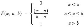
@cunif Uniform cumulative distribution function.
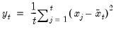
@cvar Population variance of each column of a matrix.
@cvarp Population variance of each column of a matrix.
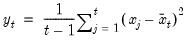
@cvars Sample variance of each column of a matrix.
@cweib Weibull cumulative distribution function.
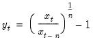
Compound annual growth rate (in decimal fraction).
Syntax: @cagr(x, n)
x: series
n: integer
Return: series
Returns the n-th root of the total return of x over n periods:
This function is panel aware.
Examples
If x is a series of quarterly profits, then
show @cagr(x, 1)
returns a linked series containing annualized profit growth rates in decimal fraction.
Cross-references
Reorder the rows of a matrix using a vector of ranks.
Syntax: @capplyranks(m, v[, n])
m: matrix, vector
v: vector
n: (optional) integer
Return: matrix, vector
Apply (a column of) row ranks in the vector v to reorder the rows of a matrix m using the ranks.
• v should contain unique integers from 1 to the number of rows of m.
• If the optional argument n is specified, only the elements in column n will be reordered.
Examples
matrix m1 = @mnrnd(10, 4)
vector v1 = @ranks(m1.@col(4), "a", "i")
matrix m2 = @capplyranks(m1, v1)
reorders the rows of the matrix M1 using the ranks in V1. Note that you may use the @ranks function to obtain the ranks of a vector, but must obtain unique integer ranking for data with ties through use of the “i” or “r” option in @ranks.
matrix m3 = @capplyranks(m1, v1, 3)
reorders only the elements of column 3 of M1.
Cross-references
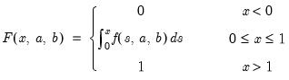
Beta distribution cumulative distribution.
Syntax: @cbeta(x, a, b[, u])
x: number
a: number,

b: number,

u: (optional) number
Return: number
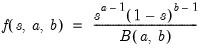
Computes the cumulative distribution function
where
and

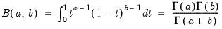
is the beta function
If the optional argument
u is non-zero, return the upper-tail value:
.
Examples
= @cbeta(0.5, 1, 2)
returns 0.75.
Cross-references
See also
@dbeta,
@qbeta, and
@rbeta.
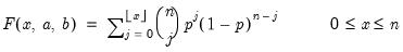
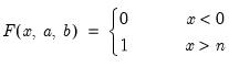
Binomial distribution cumulative probability.
Syntax: @cbinom(x, n, p)
x: number
n: integer,

p: number,

Return: number
Computes the cumulative probability function
and
where

is the integer floor of

.
Examples
= @cbinom(1, 5, 0.5)
returns 0.1875.
Cross-references
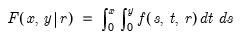
Bivariate normal cumulative probability.
Syntax: @cbvnorm(x, y, r)
x: number
y: number
p: number,

Return: number
Computes the cumulative distribution function for a bivariate normal with 0 mean, unit variances, and correlation r:
where
Examples
= @cbvnorm(0, 0, 0.5)
returns 0.33333....
Cross-references
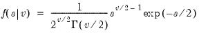
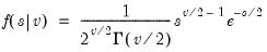
Chi-square cumulative distribution.
Syntax: @cchisq(x, v[, u])
x: number
v: number,

u: (optional) number
Return: number
Computes the cumulative distribution function
where
If the optional argument
u is non-zero, return the upper-tail value:

.
Examples
= @cchisq(100, 100)
returns 0.51880....
Cross-references
Smallest number greater than or equal to (with optional precision).
Syntax: @ceil(x[, n])
x: number
n: (optional) integer
Return: number
• @ceil(
x) returns

, the smallest integer that is greater than or equal to
x.
• @ceil(
x, n) returns
, the smallest decimal number that is greater than or equal to
x at the given precision.
The decimal offset
n may be interpreted as the precision to use when computing the ceiling. If
n is not an integer, the integer floor

will be used.
Examples
= @ceil(@pi)
returns 4.
= @ceil(@pi,2)
returns 3.15.
= @ceil(-@pi)
returns -3.
Cross-references
Panel workfile series containing within cross-section identifier for observation.
Syntax: @cellid
Return: series
Returns index of the within cross-section identifier for each observation in the workfile.
• In a panel workfile, the index numbers identify the unique values of the within cross-section dimension.
• In a non-panel workfile, the index numbers are equivalent to sequential observation numbers.
Examples
wfcreate a 2001 2022 10
series ids = @cellid
creates a balanced 10 cross-section panel, with 22 observations per cross-section, and saves a series with indices (1 to 22) corresponding to the year of the observation.
If we have an unbalanced panel
series ubids = @cellid
will contain indices uniquely identifying the values of the all of the within cross-section identifiers observed in the workfile.
Thus, in a two-cross section panel where the first cross-section has annual observations for 1990, 1992, 1994, and 1995, and the second cross-section has observations for 1990, 1995, and 1997, the corresponding index values will be of the form (1, 2, 3, 4) and (1, 4, 5), respectively.
Cross-references
See also
@obsrange,
@crossid, and
@obsid.
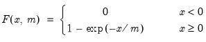
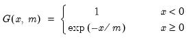
Exponential cumulative distribution.
Syntax: @cexp(x, m[, u])
x: number
m: number,

u: (optional) number
Return: number
Computes the cumulative distribution function
If the optional argument u is non-zero, return the upper-tail value:
Examples
= @cexp(@log(2), 1)
returns 0.5.
Cross-references
See also
@dexp,
@qexp, and
@rexp.
Extreme value (Type I-minimum) cumulative distribution.
Syntax: @cextreme(x, [, u])
x: number
u: (optional) number
Return: number
Computes the cumulative distribution function
If the optional argument u is non-zero, return the upper-tail value:
Examples
= @cextreme(-0.36651)
returns 0.50000....
Cross-references
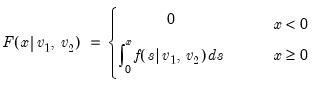
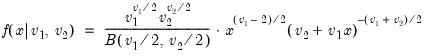
F-distribution cumulative distribution.
Syntax:
@cfdist(
x,  ,
,  [, u])
 x: number

: number,


: number,

u: (optional) number
Return: number
Computes the cumulative distribution function
where
for

and 0 otherwise, and

is the beta function
Note that the functions allow for fractional degrees of freedom parameters

and

.
If the optional argument
u is non-zero, return the upper-tail value:

.
Examples
= @cfdist(1, 2, 2)
returns 0.5.
Cross-references
First non-missing value in each column of a matrix object.
Syntax: @cfirst(m)
m: matrix
Return: vector
Returns a vector containing the first non-missing value from each column of the matrix m.
Examples
Let M1 be an

lower triangular matrix whose
elements above the main diagonal are NAs. In this case,
= @cfirst(m1)
returns the main diagonal of M1 as a column vector.
Cross-references
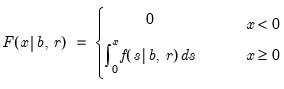
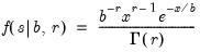
Gamma cumulative distribution.
Syntax: @cgamma(x, b, r[, u])
x: number
b: number,

r: number,

u: (optional) number
Return: number
Computes the cumulative distribution function
where
for

and 0 elsewhere.
If the optional argument
u is non-zero, return the upper-tail value:

Examples
= @cgamma(2.7725, 4, 1)
returns 0.49998....
Cross-references
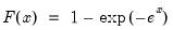
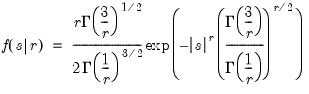
Generalized error cumulative distribution.
Syntax: @cged(x, r[, u])
x: number
r: number,

u: (optional) number
Return: number
Computes the cumulative distribution function
where
If the optional argument
u is non-zero, return the upper-tail value:

.
Examples
Cross-references
= @cged(0.675, 2)
returns 0.75016.
See also
@dged,
@qged, and
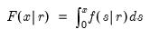
@rged.
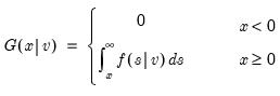
Upper tail of the Chi-square distribution.
Syntax: @chisq(x, v)
x: number
v: number,

Return: number
Returns the probability that a Chi-squared statistic with

degrees of freedom exceeds

.
Computes the upper tail of the cumulative distribution function
where
Examples
= @chisq(100, 100)
returns 0.48119....
Cross-references
Cholesky factor of matrix.
Syntax: @cholesky(s)
s: sym
Return: matrix
Returns a matrix containing the Cholesky factorization of

.
The Cholesky factorization finds the lower triangular matrix

such that

is equal to the symmetric source matrix

.
Examples
sym s = @inner(@mrnd(10, 10))
matrix chol = @cholesky(s)
matrix orig1 = chol * chol.@t
sym orig2 = @inner(chol.@t)
computes the Cholesky, and uses it to recreate the original matrix. Note that ORIG1 is a matrix object whereas ORIG2 is a sym object.
Inverting the Cholesky may be used to obtain the matrix inverse.
sym sinv1 = @inverse(s)
matrix invchol = @inverse(chol)
matrix sinv2 = invchol.@t * invchol
sym sinv3 = @inner(invchol)
matrix id1 = sinv1 * s
matrix id2 = sinv2 * s
matrix id3 = sinv3 * s
uses properties of the inverse of the Cholesky to recreate the matrix inverse so that ID1, ID2, and ID3 are all different computations yielding the identity matrix.
Cross-references
ASCII value to string character.
Syntax: @chr(arg)
arg: integer
Return: string
Returns the character string corresponding to the ASCII value arg.
Valid inputs are integer values running from 0 to 255. Any invalid value will return an empty string.
Examples
string s1 = @chr(67)
string s2 = @chr(99)
returns the strings S1=“C” and S2=“c”.
Cross-references
Index of the first non-missing value in each column of a matrix.
Syntax: @cifirst(m)
m: matrix
Return: vector
Returns a vector containing the index (i.e, row number) of the first non-missing value of each column of the matrix m.
Examples
Let M1 be an

lower triangular matrix whose

elements above the main diagonal are NAs. In this case,
= @cifirst(m1)
returns a column vector whose elements are the integers 1, 2, ...,

.
Cross-references
Index of the last non-missing value in each column of a matrix.
Syntax: @cilast(m)
m: matrix
Return: vector
Returns a vector containing the index (i.e, row number) of the last non-missing value of each column of the matrix m.
Examples
Let M2 be an

upper triangular matrix whose

elements below the main diagonal are NAs. In this case,
= @cilast(m2)
returns a column vector whose elements are the integers 1, 2, ...,

.
Cross-references
Index of the maximal value in each column of a matrix.
Syntax: @cimax(m)
m: matrix
Return: vector
Returns a vector containing the index (i.e, row number) of the maximal values of each column of the matrix m.
Examples
Let ID be an

identity matrix. Then
= @cimax(id)
returns a column vector whose elements are the integers 1, 2, ...,

.
Cross-references
See also
@cimin,
@cmax, and
@cmin.
Index of the minimal value in each column of a matrix.
Syntax: @cimin(m)
m: matrix
Return: vector
Returns a vector containing the index (i.e, row number) of the minimal values of each column of m.
Examples
Let ID be an

identity matrix. Then
= @cimin(id)
returns a column

-vector whose elements are 2, 1, 1, ..., 1, i.e., a 2 followed by

1s.
Cross-references
See also
@cimax,
@cmax, and
@cmin.
Intercept from a trend regression performed on each column of a matrix.
Syntax: @cintercept(m)
m: matrix
Return: vector
Returns a vector of intercepts from trend regressions, each the result of applying @intercept to each column of m.
Examples
vector trend = @grid(0, 10000, 10001)
matrix m1 = @hcat(1+0.5*trend, 1+2*trend) + @mnrnd(10001, 2)
= @cintercept(m1)
produces a vector of two elements, both of which should be approximately 1.
Cross-references
Laplace cumulative distribution.
Syntax: @claplace(x[, u])
x: number
u: (optional) number
Return: number
Computes the cumulative distribution integral
where
If the optional argument
u is non-zero, return the upper-tail value:

.
Examples
= @claplace(@log(2))
returns 0.75.
Cross-references
Last non-missing value in each column of the matrix.
Syntax: @clast(m)
m: matrix
Return: vector
Returns a vector containing the last non-missing value of each column of m.
Examples
Let M2 be an

upper triangular matrix whose

elements below the main diagonal are NAs. In this case,
= @clast(m2)
returns the main diagonal of M2 as a column vector.
Cross-references
Logistic cumulative distribution.
Syntax: @clogistic(x[, u])
x: number
u: (optional) number
Return: number
Computes the cumulative distribution function
If the optional argument u is non-zero, return the upper-tail value:
Examples
= @clogistic(0)
returns 0.5.
Cross-references
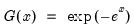
Complimentary log-log function.
Syntax: @cloglog(x)
x: number
Return: number
Compute the value of the complementary log-log function:
for

.
Examples
= @cloglog(0.5)
returns -0.36651....
Cross-references
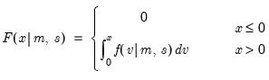
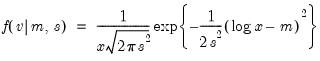
Log normal cumulative distribution.
Syntax: @clognorm(x, m, s[, u])
x: number
m: number,

s: number,

u: (optional) number
Return: number
Computes the cumulative distribution function
where
If the optional argument
u is non-zero, return the upper-tail value:
.
Examples
= @clognorm(1, 0, 2)
returns 0.5.
Cross-references
Maximal value in each column of a matrix.
Syntax: @cmax(m)
m: matrix
Return: vector
Returns a vector containing the maximal values of each column of m.
Examples
Let ID be an

identity matrix. Then
= @cmax(id)
returns a column vector of

ones.
Cross-references
See also
@cimax,
@cimin, and
@cmin.
Mean in each column of a matrix.
Syntax: @cmean(m)
m: matrix
Return: vector
Returns a vector containing the mean values of each column of the matrix m.
Examples
Let MAT be an

matrix of IID exponential numbers with mean 1. Then
= @cmean(mat)
returns an

-vector whose elements are approximately 1 for large

.
Cross-references
Median of each column of a matrix.
Syntax: @cmedian(m)
m: matrix
Return: vector
Returns a vector containing the median values of each column of m.
Examples
Let MAT be an

matrix of IID exponential numbers with mean 1. Then
= @cmean(mat)
returns an

-vector whose elements are approximately

for large

.
Cross-references
Minimal value for each column of the matrix.
Syntax: @cmin(m)
m: matrix
Return: vector
Returns a vector containing the minimal values of each column of the matrix m.
Examples
Let ID be an

identity matrix. Then
= @cmin(id)
returns a column vector of

zeros.
Cross-references
See also
@cimax,
@cimin, and
@cmax.
Number of NA values in each column of a matrix.
Syntax: @cnas(m)
m: matrix
Return: vector
Returns a vector containing the number of missing values in each column of the matrix m.
Examples
Let M1 be an

lower triangular matrix whose

elements above the main diagonal are NAs. In this case,
= @cnas(m1)
returns a column vector whose elements are the integers 0, 1, ...,

.
Cross-references
Negative binomial distribution cumulative probability.
Syntax: @cnegbin(x, n, p)
x: number
n: number,

p: number,

Return: number
Computes the cumulative probability function
and
where

is the integer floor of

.
Examples
= @cnegbin(9, 10, 0.5)
returns 0.5.
Cross-references
Standard normal cumulative distribution.
Syntax: @cnorm(x[, u])
x: number
u: (optional) number
Return: number
Computes the cumulative distribution integral
where
If the optional argument
u is non-zero, return the upper-tail value:

.
Examples
= @cnorm(-1.96)
returns 0.02499....
Cross-references
Number of non-NA values in each column of a matrix.
Syntax: @cobs(m)
m: matrix
Return: vector
Returns a vector containing the number of non-missing values in each column of the matrix m.
Examples
Let M1 be an

lower triangular matrix whose

elements above the main diagonal are NAs. In this case,
= @cobs(m1)
returns a column vector whose elements are the integers

,

, ..., 1.
Cross-references
Cumulative products for each column of a matrix.
Syntax: @colcumprod(m)
m: matrix, vector
Return: matrix, vector
Returns a matrix where each column contains the cumulative products of the values of the corresponding column of m.
For each element of the output, compute the cumulative product of the values in m from the start of the column up to the current row:
Note that this function is prone to numeric overflow.
Examples
Let M1 be an

matrix of IID uniform numbers drawn from the unit interval. Then
= @colcumprod(m1)
generates an

matrix whose

columns converge to 0 at an exponential rate.
Cross-references
See also
@cumprod and
@cumsum.
See also
@cprod,
@csum, and
@csumsq.
Cumulative sums for each column of a matrix.
Syntax: @colcumsum(m)
m: matrix, vector
Return: matrix, vector
Returns a matrix where each column contains the cumulative sums of the values of the corresponding column of m.
For each element of the output, compute the cumulative sum of the values in m from the start of the column up to the current row:
Examples
Let M1 be an

matrix of IID uniform numbers drawn from the unit interval. Then
= @colcumsum(m1)
generates an

matrix whose

columns diverge to infinity at a linear rate.
Cross-references
See also
@cumprod and
@cumsum.
See also
@cprod,
@csum, and
@csumsq.
Demean each column of a matrix.
Syntax: @coldemean(m)
m: matrix
Return: matrix
Returns the matrix containing the results from subtracting the column mean from each column of m.
For each element of the output matrix

:
for

the mean of column

where
 | (18.1) |
where

is the number of non-missing values in the column. If there are missing values in a column, they are ignored and the number of rows is adjusted.
Examples
matrix m1 = @mnrnd(50, 4)
matrix m1d = @coldemean(m1)
demeans each column of M1 and places the results in M1D.
This operation is equivalent to
vector m1means = @cmeans(m1)
matrix m2d = m1 - @kronecker(@ones(m1.@rows), m1means.@t)
where @cmeans is used to compute the column means of M1.
Cross-references
Detrend each column of a matrix.
Syntax: @coldetrend(m)
m: matrix
Return: matrix
Returns the matrix containing the results from detrending each column of m.
Detrending produces the residuals of the OLS regression of the data in column

versus an intercept and implicit time trend. For each element of the output matrix

:
where

and

are the intercept and slope coefficients of a regression of the data in column

on a constant and time trend. If there are missing values in a column, they are ignored.
Examples
matrix m1 = @mnrnd(50, 4)
matrix m1d = @coldetrend(m1)
detrends each column of M1 and places the results in M1D.
This operation is equivalent to
vector cintercepts = @cintercept(m1)
vector ctrendcs = @ctrendcoef(m1)
matrix m2d = m1 - @kronecker(@ones(m1.@rows), cintercepts.@t) - @kronecker(@range(0, m1.@rows-1), ctrendcs.@t)
where @cintercept and @ctrendcoef are used to compute the coefficients of the column trend regressions.
Cross-references
Percentile values for each column of a matrix.
Syntax: @colpctiles(m[, o])
m: matrix, vector
o: (optional) string
Return: matrix, vector
Returns a matrix where each column contains the percentiles of the values of the corresponding column of m
The option o controls the direction of the ranking: “a” (ascending - default) or “d” (descending).
Examples
Let MAT be a matrix with two columns. Then
= @colpctiles(mat)
and
= @hcat(@pctiles(mat.@col(1)), @pctiles(mat.@col(2)))
are equivalent.
Cross-references
Ranks of each column of the matrix.
Syntax: @colranks(m[, o, t])
m: matrix, vector
o: (optional) string
t: (optional) string
Return: matrix, vector
Returns a matrix where each column contains the ranks of the values of the corresponding column of m.
The o option controls the direction of the ranking:
• “a” (ascending - default) or “d” (descending).
The t option controls tie-handling:
• Ties are broken according to the setting of t: “i” (ignore), “f” (first), “l” (last), “a” (average - default), “r” randomize.
If you wish to specify tie-handling options, you must also specify the order option (e.g., @colranks(x, "a", "i")).
Examples
= @colranks(m1, "d")
returns a matrix whose i-th column ranks the elements in the i-th column of M1 so that the largest element in said column has a rank of 1.
Cross-references
See also
@ranks and
@rowranks.
Sort each column of the matrix.
Syntax: @colsort(m[, o])
m: matrix, vector
o: (optional) string
Return: matrix, vector
Returns a matrix where each column contains the sorted values of the corresponding column of m.
The option o controls the direction of the ranking: “a” (ascending - default) or “d” (descending).
Examples
Let M1 be a matrix. Then
= @colsort(m1, "d")
returns a matrix whose i-th column is the sorted (from largest at the top to smallest at the bottom) version of the i-th column in M1.
Cross-references
See also
@sort and
@rowsort.
Standardize each column using the sample (d.f. corrected) standard deviation.
Syntax: @colstdize(m)
m: matrix, vector
Return: matrix, vector
Returns the matrix containing the results from standardizing each column of m.
For each element of the output:
for

the mean and

the sample (d.f. corrected) standard deviation of column

where
 | (18.2) |
where

is the number of non-missing values in the column. If there are missing values in a column, they are ignored and the number of rows is adjusted.
Examples
matrix m1 = @mnrnd(50, 4)
matrix m1s = @colstdize(m1)
standardizes each column of M1 and places the results in M1D.
Cross-references
Standardize each column using the population (non-d.f. corrected) standard deviation.
Syntax: @colstdizep(m)
m: matrix, vector
Return: matrix, vector
Returns the matrix containing the results from standardizing each column of m.
For each element of the output:
for

the mean and

the population (non-d.f. corrected) standard deviation of column

where
 | (18.3) |
where

is the number of non-missing values in the column. If there are missing values in a column, they are ignored and the number of rows is adjusted.
Examples
matrix m1 = @mnrnd(50, 4)
matrix m1s = @colstdizep(m1)
standardizes each column of M1 and places the results in M1D.
Cross-references
Extract a column from the matrix.
Syntax: @columnextract(m, n)
m: matrix, sym
n: integer
Return: vector
Extract a vector from column n of the matrix object m, where m is a matrix object.
Note that we recommend that extraction be performed using the newer “.col” object data member functions. See
“Matrix Data Members” and
“Sym Data Members” and the examples below.
Examples
matrix m1 = @mnrnd(20, 5)
vector v1 = @columnextract(m1,3)
extracts column 3 from the matrix M1.
sym s1 = @mnrnd(5, 5)
vector v2 = @columnextract(s1, 5)
Alternately, using the data member functions, we have
vector v1a = m1.@col(3)
vector v2a = s1.@col(5)
Cross-references
Number of columns in matrix object or group.
Syntax: @columns(x)
m: matrix, sym, group
Return: integer
Examples
matrix m1 = @mnrnd(10, 3)
scalar sc1 = @columns(m1)
assigns the value 3 to the scalar object SC1.
Cross-references
Commutation matrix.
Syntax: @commute(m, n)
m: integer
n: integer
Return: matrix
The commutation matrix transforms the vectorization of a matrix to the vectorization of its transpose.
Given the

matrix

, returns the

matrix

, which satisfies
Examples
matrix m1 = @mnrnd(10, 5)
vector diff = @commute(10, 5) * @vec(m1) - @vec(m1.@t)
demonstrates the properties of the commutation matrix since DIFF equals zero.
Cross-references
Condition number of matrix.
Syntax: @cond(m[, n])
m: matrix, sym
n: (optional) integer
Return: number
Returns the condition number of a square matrix or sym, m.
The condition number is the product of the norm of the matrix divided by the norm of the inverse.
If the norm option
n is omitted, the infinity norm is used to determine the condition number. Possible norms are “-1” for the infinity norm, “0” for the Frobenius norm, and an integer “n” for the

norm.
Examples
matrix m1 = @mnrnd(10, 10)
scalar sc1 = @cond(m1)
computes the infinity norm of the matrix M1.
sym s1 = @inner(m1)
scalar sc2 = @cond(s1, 2)
computes the

norm of the symmetric matrix S1.
Cross-references
Converts series, alpha, or group to matrix objects after removing NAs.
Syntax: @convert(o[, s])
o: series, alpha, group
s: (optional) sample string or object
Return: vector, svector, matrix
Convert data in the series (numeric or alpha) or group object into a vector (numeric or alpha) or group after removing rows with an NA or “”.
• If o is a series, @convert returns a vector from the values of o using the optional sample s or the current workfile sample. If any observation has the value “NA”, the observation will be omitted from the vector.
• If o is an alpha series, @convert returns an svector from the values of o using the optional sample s or the current workfile sample.
• If o is a group, @convert returns a matrix from the values of o using the optional sample object smp or the current workfile sample.
The data for series in o are placed in the columns of the resulting matrix in the order they appear in the group spreadsheet. If any of the series for a given observation has the value “NA”, the observation will be omitted for all series.
Note that if the group contains alpha series, they are treated as numeric series with all NA values for purposes of this conversion.
For a conversion method that preserves NAs, see
stomna.Examples
vector v2 = @convert(ser1)
vector v3 = @convert(ser2, "2000m12 2022m01")
converts the numeric series SER1 and SER2 into the vectors V2 and V3. V2 contains all non-missing elements in the current workfile sample, while V3 contains non-missing elements from 2000m12 to 2022m01.
sample smpl "2000m10 2022m05"
svector a2 = @convert(alp1)
svector a3 = @convert(alp2, smpl)
converts the alpha series ALP1 and ALP2 into the svectors A2 and A3. A2 contains all non-missing (non-blank) elements in the current workfile sample, while A3 contains non-missing elements from 2000m10 to 2022m05.
matrix m1 = @convert(grp1)
matrix m2 = @convert(grp1, smpl)
converts the series in the group GRP1 into the matrices M1 and M2.
M1 uses all non-missing observations in the current workfile sample, while M2 uses non-missing observations in the sample object from 2000m10 to 2022m05. Note that if GRP1 contains alpha series, they are treated as numeric series with all NA values for purposes of this conversion.
Cross-references
Computes the correlation between two vectors, or between the columns of a matrix.
Syntax: @cor(x, y)
x: vector, rowvector, or series
y: vector, rowvector, or series
Return: scalar
Syntax: @cor(m)
m: matrix object or group
Return: sym
For series and group calculations, EViews will use the current workfile sample.
Examples
If used with two vector or series objects, @cor returns the correlation between the two vectors or series.
scalar sc1 = @cor(v1, v2)
If used with a matrix object or group, @cor calculates the correlation matrix between the columns of the matrix object or the series in the group object.
sym s1 = @cor(mat1)
Cross-references
See also
@cov,
@covp, and
@covs.
Cosine of argument specified in radians.
Compute the cosine of x (specified in radians).
Syntax: @acos(x)
x: number
Return: number
Examples
= @cos(@pi)
returns -1.
Cross-references
Compute population (non-d.f. corrected) covariance between two vectors, or between the columns of a matrix.
Syntax: @cov(v1, v2)
v1: vector, rowvector, or series
v2: vector, rowvector, or series
Return: scalar
Syntax: @cov(o)
o: matrix object or group
Return: sym
Compute covariances using

as the divisor in the moment calculation.
For series and group calculations, EViews will use the current workfile sample.
Examples
If used with two vector or series objects, @cov returns the population covariance between the two vectors or series.
scalar sc1 = @cov(v1, v2)
If used with a matrix object or group, @cov calculates the population covariance matrix between the columns of the matrix object or the series in the group object.
sym s1 = @cov(mat1)
Cross-references
See also
@cor,
@covp, and
@covs.
Compute population (non-d.f. corrected) covariance between two vectors, or between the columns of a matrix.
Syntax: @covp(v1, v2)
v1: vector, rowvector, or series
v2: vector, rowvector, or series
Return: scalar
Syntax: @covp(o)
o: matrix object or group
Return: sym
Compute covariances using

as the divisor in the moment calculation.
For series and group calculations, EViews will use the current workfile sample.
Examples
If used with two vector or series objects, @covp returns the population covariance between the two vectors or series.
scalar sc1 = @covp(v1, v2)
If used with a matrix object or group, @covp calculates the population covariance matrix between the columns of the matrix object.
sym s1 = @covp(mat1)
Cross-references
See also
@cor,
@cov, and
@covs.
Compute sample (d.f. corrected) covariance between two vectors, or between the columns of a matrix.
Syntax: @covs(v1, v2)
v1: vector, rowvector, or series
v2: vector, rowvector, or series
Return: scalar
Syntax: @covs(o)
o: matrix object or group
Return: sym
Compute covariances using

as the divisor in the moment calculation.
For series and group calculations, EViews will use the current workfile sample.
Examples
If used with two vector or series objects, @covs returns the sample covariance between the two vectors or series.
scalar sc1 = @covs(v1, v2)
If used with a matrix object or group, @covs calculates the sample covariance matrix between the columns of the matrix object.
sym s1 = @covs(mat1)
Cross-references
See also
@cor,
@cov, and
@covp.
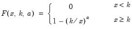
Pareto cumulative distribution.
Syntax: @cpareto(x, k, a[, u])
x: number
k: number,

a: number,

u: (optional) number
Return: number
Computes the cumulative distribution function
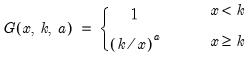
If the optional argument u is non-zero, return the upper-tail value:
Examples
= @cpareto(2, 1, 2)
returns 0.75.
Cross-references
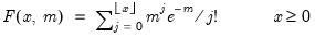
Poisson distribution cumulative probability.
Syntax: @cpoisson(x, m)
x: number
m: number,

Return: number
Computes the cumulative probability function
and
where

is the integer floor of

.
Examples
= @cpoisson(10, 10)
returns 0.58303....
Cross-references
Product of elements in each column of a matrix.
Syntax: @cprod(m)
m: matrix
Return: vector
Returns a vector containing the column products. One should be aware of overflow.
Examples
vector colprods = @cprod(m1)
computes the column products for the matrix M1 and places them in COLPRODS.
Cross-references
See also
@cumprod and
@cumsum.
See also
@csum and
@csumsq.
Quantiles for each column of a matrix.
Syntax: @cquantile(m, q)
m: matrix
q: number
Return: vector
Returns the column q-quantile using the Cleveland definition. q must be between zero and one.
Examples
Let M1 be a matrix. Then
= @cquantile(m1, .5)
and
= @cmedian(m1)
are equivalent.
Cross-references
Panel workfile series containing cross-section identifier (index) for observation.
Syntax: @crossid
Return: series
Returns the index of the cross-section identifier for each observation in the workfile.
• In a panel workfile, the index numbers identify the cross-section.
• In a non-panel workfile, there is a single cross-section, so the function returns 1.
Examples
wfcreate a 2001 2022 10
series ids = @crossid
returns a series with integer index values identifying the cross-section.
If you have an unbalanced panel,
series ids = @crossid
ids.freq
displays a one-way tabulation of the cross-section ids, so that you can see the number of observations in each cross-section.
Cross-references
Sample standard deviation (d.f. corrected) of each column of a matrix.
Syntax: @cstdev(m)
m: matrix
Return: vector
Returns the column sample standard deviation.
Examples
= @cstdev(mat)
returns a (column) vector whose i-th element is the sample standard deviation of the i-th column of MAT.
Cross-references
See also
@cmean and
@cstdevs.
Population standard deviation (non-d.f. corrected) of each column of a matrix.
Syntax: @cstdevp(m)
m: matrix
Return: vector
Returns the column population standard deviation.
Examples
= @cstdevp(mat)
returns a (column) vector whose i-th element is the population standard deviation of the i-th column of MAT.
Cross-references
See also
@cstdev and
@cstdevs.
Sample standard deviation (d.f. corrected) of each column of a matrix
Syntax: @cstdevs(m)
m: matrix
Return: vector
Returns the column sample standard deviation.
Examples
= @cstdevs(mat)
returns a (column) vector whose i-th element is the sample standard deviation of the i-th column of MAT.
Cross-references
See also
@cstdev and
@cstdevp.
Sum of the values in each column of a matrix.
Syntax: @csum(m)
m: matrix
Return: vector
Returns a vector containing the summation of the rows in each column of the matrix m.
Examples
vector colsums = @csum(m1)
computes the column sums for the matrix M1 and places them in COLSUMS.
Cross-references
See also
@cumprod and
@cumsum.
See also
@cprod and
@csumsq.
Sum of the squared values in each column of a matrix.
Syntax: @csumsq(m)
m: matrix
Return: vector
Returns the sum of squared values for each column of m.
Examples
vector colsumsqs = @csumsq(m1)
computes the column sums-of-squares for matrix M1 and places them in COLSUMSQS.
Cross-references
See also
@cumprod and
@cumsum.
See also
@cprod and
@csum.
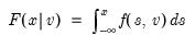
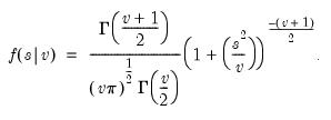
Student’s

cumulative distribution.
Syntax: @ctdist(x, v[, u])
x: number
v: number,

u: (optional) number
Return: number
Computes the cumulative distribution function
where
If the optional argument
u is non-zero, return the upper-tail value:

.
Note that  , yields the Cauchy distribution.
 Examples
= @ctdist(-12.71, 1)
returns 0.02499....
Cross-references
Slope from a trend regression on each column of a matrix.
Syntax: @ctrendcoef(m)
m: matrix
Return: vector
Returns a vector of slopes from a trend regression, each the result of applying @trendcoef to the columns of m.
Examples
vector trend = @grid(0, 10000, 10001)
matrix m1 = @hcat(1+0.5*trend, 1+2*trend) + @mnrnd(10001, 2)
= @ctrendcoef(m1)
produces a vector of two elements, the first of which should be close to 0.5, the second of which should be approximately 2.
Cross-references
Trimmed mean of each column of a matrix.
Syntax: @ctrmean(m, p)
m: matrix
p: number
Return: vector
Returns a vector of trimmed means, each the result of applying @trmean to columns of m.
Examples
matrix m = @mrnd(100,10)
m(1,1) = 1000
= @cmean(m)
returns a vector of column means of M, the first of which should be approximately 10.495, the rest of which should be around 0.5.
= @ctrmean(m,1)
returns a vector of trimmed column means of M, all of which should be approximately 0.5.
Cross-references
Backward cumulative maximums of a series.
Decreasing samples calculation of the maximum.
Syntax: @cumbmax(x, [s])
x: series
s: (optional) sample string or object
Return: series
The backward maximum for each observation

may be written as the maximum value from the current observation to the last period, so that
where the order statistics

represent data for the

observations (

), ordered from low to high, where

is the last period.This function is panel aware.
Examples
show @cumbmax(x)
generates a linked series of the backward cumulative maximum of the series x.
Cross-references
For the forward variant of this function, see
@cummax.
Backward cumulative means of a series.
Decreasing samples calculation of the mean of the values in x.
Syntax: @cumbmean(x[, s])
x: series
s: (optional) sample string or object
Return: series
Compute the mean of the values in
x from

to the end of the workfile or from

to the end of the optional sample
s:
where

is the last period of the cumulative process, and

.
This function is panel aware.
Examples
show @cumbmean(x)
generates a linked series of the backward cumulative mean of the observations in series x.
Cross-references
For the forward variant of this function, see
@cummean.
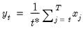
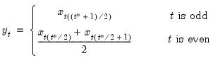
Backward cumulative median of a series.
Decreasing samples calculation of the median.
Syntax: @cumbmedian(x, [s])
x: series
s: (optional) sample string or object
Return: series
The median for each observation

may be written as:
where order statistics

represent data for the

observations (

), ordered from low to high, and

is the last period.
This function is panel aware.
Examples
show @cumbmedian(x)
generates a linked series of the backward cumulative median of the series x.
Cross-references
For the forward variant of this function, see
@cummedian.
Backward cumulative minimum of a series.
Decreasing samples calculation of the minimum.
Syntax: @cumbmin(x, [s])
x: series
s: (optional) sample string or object
Return: series
The backward maximum as the minimum value from the current observation to the end of the sample, so that:
where the order statistics
represent data for the

observations (

), ordered from low to high, and

is the last period.
This function is panel aware.
Examples
show @cumbmin(x)
generates a linked series of the backward cumulative minimum of the series x.
Cross-references
For the forward variant of this function, see
@cummin.
Backward cumulative missing observations of a series.
Increasing samples calculation of the missing (NA) observations
in  .
.Syntax: @cumbnas(x[, s])
x: series
s: (optional) sample string or object
Return: series
Compute the number of missing (NA) values in
x from

to the end of the workfile or from

to the end of the optional sample
s.
This function is panel aware.
Examples
series x = @recode(@rnd > 0.5, @nrnd, na)
show x @cumbnas(x)
produces a spreadsheet with two columns correspond to x and @cumbnas(x). The second series (which corresponds to @cumbnas(x)) starts at the count returned by @nas(x) and decrements in those observations where x is NA.
Cross-references
For the forward variant of this function, see
@cumnas.
Backward cumulative observations of a series.
Increasing samples calculation of the number of non-missing observations
in  .
.Syntax: @cumbobs(x[, s])
x: series
s: (optional) sample string or object
Return: series
Compute the number of non-missing values in
x from

to the end of the workfile or from

to the end of the optional sample
s.
This function is panel aware.
Examples
series x = @recode(@rnd > 0.5, @nrnd, na)
show x @cumbobs(x)
produces a spreadsheet with two columns correspond to x and @cumbobs(x). The second series (which corresponds to @cumbobs(x)) starts at the count returned by @obs(x) and decrements in those observations where x is non-NA.
Cross-references
For the forward variant of this function, see
@cumobs.
Backward cumulative products of a series.
Decreasing samples calculation of the product of the values in x.
Syntax: @cumbprod(x[, s])
x: series
s: (optional) sample string or object
Return: series
Compute the product of the values in
x from

to the end of the workfile or from

to the end of the optional sample
s:
where

is the last period of the cumulative process. Note that this function is prone to numeric overflow.
This function is panel aware.
Examples
show @cumbprod(x)
generates a linked series of the backward cumulative product of the observations in series x.
Cross-references
For the forward variant of this function, see
@cumprod.
Cumulative quantiles of a series.
Increasing samples calculation of the quantile value where approximately 100*q percent of the data is less than or equal to the value,
Syntax: @cumbquantile(x, q, [s])
x: series
q: number, series
s: (optional) sample string or object
Return: series
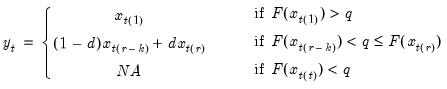
• The quantile value
q must satisfy

.
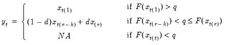
• The cumulative quantiles are computed using the Rankit-Cleveland definition of the empirical distribution function:
.
To compute the cumulative backward quantile for observation

find

, the smallest rank such that:
where the order statistics

represent data for the

observations (

), ordered from low to high, and

is the last period. For purposes of computing

, tied ranks are assumed to take the last tied value.
Then the quantile is computed as:
where the interpolating constant is
for

the smallest integer where
. In the leading case where there are no tied

values,

.
This function is panel aware.
Examples
show @cumbquantile(x, 0.1)
generates a linked series of the backward cumulative 10th percentile of the series x.
Cross-references
For the forward variant of this function, see
@cumquantile.
Backward cumulative standard deviations (d.f. adjusted) of a series.
Equivalent to @cumbstdevs.
Decreasing sample calculation of the square root of the sample (d.f. adjusted) Pearson product moment variance.
Syntax: @cumbstdev(x, [s])
x: series
s: (optional) sample string or object
Return: series
The sample standard deviation is calculated for each observation

as:
where

is the last period of the cumulative process,

, and

is the mean of

over the last

observations.
Examples
show @cumbstdev(x)
generates a linked series of the backward cumulative sample standard deviations of the series x.
Cross-references
For the forward variant of this function, see
@cumstdev.
Backward cumulative standard deviations (population, non-d.f. corrected).
Decreasing samples calculation of the square root of the population (non-d.f. adjusted) Pearson product moment variance.
Syntax: @cumbstdevp(x, [s])
x: series
s: (optional) sample string or object
Return: series
The population standard deviation is calculated for each observation

as:
where

is the last period of the cumulative process,

, and

is the mean of

over the last

observations.
This function is panel aware.
Examples
show @cumbstdevp(x)
generates a linked series of the backward cumulative population standard deviations of the series x.
Cross-references
For the forward variant of this function, see
@cumstdevp.
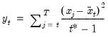
Backward cumulative sample standard deviations (sample, d.f. corrected) of a series.
Decreasing sample calculation of the square root of the sample (d.f. corrected) Pearson product moment variance.
Syntax: @cumbstdevs(x, [s])
x: series
s: (optional) sample string or object
Return: series
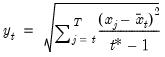
The sample standard deviation is calculated for each observation

as:
where

is the last period of the cumulative process,

, and

is the mean of

over the last

observations.
This function is panel aware.
Examples
show @cumbstdevs(x)
generates a linked series of the backward cumulative sample standard deviations of the series x.
Cross-references
For the forward variant of this function, see
@cumstdevs.
Backward cumulative sums of a series.
Decreasing samples calculation of the sum of the values in x.
Syntax: @cumbsum(x[, s])
x: series
s: (optional) sample string or object
Return: series
Compute the sum of the values in
x from

to the end of the workfile or from

to the end of the optional sample
s:
where

is the last period of the cumulative process.
This function is panel aware.
Examples
show @cumbsum(x)
generates a linked series of the backward cumulative sum of the observations in series x.
Cross-references
For the forward variant of this function, see
@cumsum.
Backward cumulative sums of squares of a series.
Decreasing samples calculation of the sum of the squared values in x.
Syntax: @cumbsumsq(x[, s])
x: series
s: (optional) sample string or object
Return: series
Compute the sum of the squared values in
x from

to the end of the workfile or from

to the end of the optional sample
s:
where  is the last period of the cumulative process.
 This function is panel aware.
Examples
show @cumbsumsq(x)
generates a linked series of the backward cumulative sums of squares of the series x.
Cross-references
For the forward variant of this function, see
@cumsumsq.
Backward cumulative variances (non-d.f. corrected) of a series.
Equivalent to @cumbvarp.
Decreasing samples calculation of the population (non-d.f. corrected) Pearson product moment variance.
Syntax: @cumbvar(x, [s])
x: series
s: (optional) sample string
Return: series
The population variance for each observation

is calculated as:
where

is the last period of the cumulative process,

, and

is the mean of

over the last

observations.
This function is panel aware.
Examples
show @cumbvar(x)
generates a linked series of the backward cumulative population variance of the series x.
Cross-references
For the forward variant of this function, see
@cumvar.
Backward cumulative variance (population, non-d.f. corrected) of a series.
Decreasing samples calculation of the population (non-d.f. corrected) Pearson product moment variance.
Syntax: @cumbvarp(x, [s])
x: series
s: (optional) sample string
Return: series
The population variance for each observation

is calculated as
where

is the last period of the cumulative process,

, and

is the mean of

over the last

observations.
Examples
show @cumbvarp(x)
generates a linked series of the backward cumulative population variance of the series x.
Cross-references
For the forward variant of this function, see
@cumvarp.
Backward cumulative variances (sample, d.f. corrected) of a series.
Decreasing samples calculation of the sample (d.f. corrected) Pearson product moment variance.
Syntax: @cumbvars(x, [s])
x: series
s: (optional) sample string or object
Return: series
The sample variance for each observation

is calculated as:
where

is the last period of the cumulative process,
, and

is the mean of

over the last

observations.
This function is panel aware.
Examples
show @cumbvars(x)
generates a linked series of the backward cumulative sample variance of the series x.
Cross-references
For the forward variant of this function, see
@cumvars.
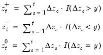
Cumulative process of negative (below threshold) changes.
Compute the partial sum process of negative (below the threshold y) changes in the series beginning in the specified date.
Syntax: @cumdn(x, d[, y, s])
x: series
d: string
y: (optional) number
s: (optional) sample string or object
Return: series
Consider the partial sum decomposition of a variable

given a initial value

as

where

,

, and

are the partial sum processes of the differences for positive, negative, and zero
changes in

relative to the threshold
y:
This function returns the negative partial sums

for the current or specified sample.
• The date
d specification determines

.
• Values for dates prior to d will be NAs.
• The optional

argument specifies the threshold value. By default

.
This function is panel aware.
Examples
The code below produces a graph of a sine wave x and @cumdn applied on x.
wfcreate u 50
series x = @sin(@pi*@trend/4)
group g x @cumdn(x,1)
g.line
Cross-references
Cumulative process of positive (above threshold) changes.
Compute the partial sum process of positive (above the threshold y) changes in the series x beginning in the specified date.
Syntax: @cumdp(x, d[, y, s])
x: series
d: string
y: (optional) number
s: (optional) sample string or object
Return: series
Consider the partial sum decomposition of a variable

given a initial value

as

where

,

, and

are the partial sum processes of the differences for positive, negative, and zero
changes in

relative to the threshold
y:
This function returns the positive partial sums

for the current or specified sample.
• The date
d string specification determines

.
• Values for dates prior to d will be NAs.
• The optional

argument specifies the threshold value. By default

.
This function is panel aware.
Examples
The code below produces a graph of a sine wave x and @cumdp applied on x.
wfcreate u 50
series x = @sin(@pi*@trend/4)
group g x @cumdp(x,1)
g.line
Cross-references
Cumulative process of zero (at threshold) changes.
Compute the partial sum process of positive (at the threshold y) changes in the series x beginning in the specified date.
Syntax: @cumdz(x, d[, y, s])
x: series
d: string
y: (optional) number
s: (optional) sample string or object
Return: series
Consider the partial sum decomposition of a variable

given a initial value

as
where

,

, and

are the partial sum processes of the differences for positive, negative, and zero
changes in

relative to the threshold
y:
This function returns the zero change

for the current or specified sample.
• The date
d string specification determines

.
• Values for dates prior to d will be NAs.
• The optional

argument specifies the threshold value. By default

.
This function is panel aware.
Examples
show @cumdz(x, 2001, 1)
produces a linked series of @cumdz applied to x where the starting date is 2001 and the threshold value is set to 1.
Cross-references
Cumulative maximum of a series.
Increasing samples calculation of the maximum.
Syntax: @cummax(x, [s])
x: series
s: (optional) sample string or object
Return: series
The maximum for each observation

may be written as
where the order statistics
represent data from the beginning of the workfile or sample
s, up to the current observation (

), ordered from low to high.
This function is panel aware.
Examples
series x = @cummax(@rnd)
generates a random process x that converges in probability to 1.
Cross-references
For the backward variant of this function, see
@cumbmax.
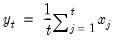
Cumulative means of a series.
Increasing samples calculation of the mean of the values in x.
Syntax: @cummean(x[, s])
x: series
s: (optional) sample string or object
Return: series
Compute the cumulative mean of the values in x from the start of the workfile or sample s, up to the current observation:
This function is panel aware.
Examples
series x = @cummean(@nrnd)
generates a random process x that converges in probability to 0.
Cross-references
For the backward variant of this function, see
@cumbmean.
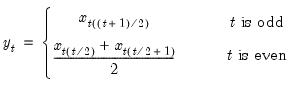
Cumulative median of a series.
Increasing samples calculation of the median.
Syntax: @cummedian(x, [s])
x: series
s: (optional) sample string or object
Return: series
The median for each observation

may be written as
where the order statistics
represent data from the beginning of the workfile or sample
s, up to the current observation (

), ordered from low to high.
This function is panel aware.
Examples
series x = @cummedian(@rnd)
generates a random process x that converges in probability to 0.5.
Cross-references
For the backward variant of this function, see
@cumbmedian.
Cumulative minimum of a series.
Increasing samples calculation of the minimum.
Syntax: @cummin(x, [s])
x: series
s: (optional) sample string or object
Return: series
The minimum for each observation

may be written as
where the order statistics

represent data from the beginning of the workfile or sample
s, up to the current observation (

), ordered from low to high.
This function is panel aware.
Examples
series x = @cummin(@rnd)
generates a random process x that converges in probability to 0.
Cross-references
For the backward variant of this function, see
@cumbmin.
Cumulative missing observations of a series.
Increasing samples calculation of the missing (NA) observations
in  .
.Syntax: @cumnas(x[, s])
x: series
s: (optional) sample string or object
Return: series
Compute the number of missing (NA) values in x from the start of the workfile or sample s, up to the current observation.
This function is panel aware.
Examples
series x = @recode(@rnd > 0.5, @nrnd, na)
show x @cumnas(x)
produces a spreadsheet with two columns correspond to x and @cumnas(x). The second series (which corresponds to @cumnas(x)) starts at 0 (if the first observation in x is non-NA) or 1 (if the first observation in x is NA) and increments in those observations where x is NA.
Cross-references
For the backward variant of this function, see
@cumbnas.
Cumulative observations of a series.
Increasing samples calculation of the number of non-missing observations
in  .
.Syntax: @cumobs(x[, s])
x: series
s: (optional) sample string or object
Return: series
Compute the number of non-missing values in x from the start of the workfile or sample s, up to the current observation.
This function is panel aware.
Examples
series x = @recode(@rnd > 0.5, @nrnd, na)
show x @cumobs(x)
produces a spreadsheet with two columns correspond to x and @cumobs(x). The second series (which corresponds to @cumobs(x)) starts at 0 (if the first observation in x is NA) or 1 (if the first observation in x is non-NA) and increments in those observations where x is non-NA.
Cross-references
For the backward variant of this function, see
@cumbobs.
Cumulative products of a series or of the elements of a matrix.
• Compute the cumulative product of the values in the series x from the start of the workfile or sample s, up to the current observation:
Syntax: @cumprod(x[, s])
x: series, matrix, vector
s: (optional) sample string or object
Return: series, matrix, vector
• Compute the cumulative product of the elements of the matrix in vec order.
Syntax: @cumprod(m)
m: matrix, vector
Return: matrix, vector
This function is panel aware.
Note that this function is prone to numeric overflow.
Examples
show @cumprod(x)
produces a linked series whose elements are the cumulative products of the elements in x.
Cross-references
For the backward variant of this function for series, see
@cumbprod.
Cumulative quantiles of a series.
Increasing samples calculation of the quantile value where approximately 100*q percent of the data is less than or equal to the value,
Syntax: @cumquantile(x, q, [s])
x: series
q: number, series
s: (optional) sample string or object
Return: series
• The quantile value
q must satisfy

.
• The cumulative quantiles are computed using the Rankit-Cleveland definition of the empirical distribution function: for observation

,

.
To compute the cumulative quantile for observation

find

, the smallest rank such that:
where the order statistics

represent data from the beginning of the workfile or sample
s, up to the current observation (

), ordered from low to high. For purposes of computing

, tied ranks are assumed to take the last tied value.
Then the quantile is computed as
where the interpolating constant is
for

the smallest integer where

. In the leading case where there are no tied

values,

.
This function is panel aware.
Examples
show @cumquantile(@nrnd, 0.975)
generates a linked series that converges in probability to 1.95996... (the 97.5th percentile of the standard normal distribution).
Cross-references
For the backward variant of this function, see
@cumbquantile.
Cumulative standard deviations (d.f. adjusted) of a series.
Equivalent to @cumstdevs.
Increasing samples calculation of the square root of the sample (d.f. adjusted) Pearson product moment variance.
Syntax: @cumstdev(x, [s])
x: series
s: (optional) sample string or object
Return: series
The sample standard deviation is calculated for each observation

as
where

is the mean of

over the first

observations.
This function is panel aware.
Examples
series x = @nrnd
group g @cumstdev(x) @cumstdevs(x) @cumstdevp(x)
g.line
plots @cumstdev(x), @cumstdevs(x), and @cumstdevp(x) together. Note that @cumstdev(x) and @cumstdevp(x) are equivalent. All three series converge in probability to 1.
Cross-references
For the backward cumulative variant of this function, see
@cumbstdev.
Cumulative standard deviations (population – non-d.f. adjusted).
Increasing samples calculation of the square root of the population (non-d.f. adjusted) Pearson product moment variance.
Syntax: @cumstdevp(x, [s])
x: series
s: (optional) sample string or object
Return: series
The population standard deviation is calculated for each observation

as
where

is the mean of

over the first

observations.
This function is panel aware.
Examples
series x = @nrnd
group g @cumstdev(x) @cumstdevs(x) @cumstdevp(x)
g.line
plots @cumstdev(x), @cumstdevs(x), and @cumstdevp(x) together. Note that @cumstdev(x) and @cumstdevp(x) are equivalent. All three series converge in probability to 1.
Cross-references
For the backward variant of this function, see
@cumbstdevp.
Cumulative sample standard deviations (sample – d.f. adjusted) of a series.
Increasing samples calculation of the square root of the sample (d.f. adjusted) Pearson product moment variance.
Syntax: @cumstdevs(x, [s])
x: series
s: (optional) sample string or object
Return: series
The sample standard deviation is calculated for each observation

as
where

is the mean of

over the first

observations.
This function is panel aware.
Examples
series x = @nrnd
group g @cumstdev(x) @cumstdevs(x) @cumstdevp(x)
g.line
plots @cumstdev(x), @cumstdevs(x), and @cumstdevp(x) together. Note that @cumstdev(x) and @cumstdevp(x) are equivalent. All three series converge in probability to 1.
Cross-references
For the backward variant of this function, see
@cumbstdevsCumulative sums of a series or of the elements of a matrix.
• Compute the sum of the values in the series x from the start of the workfile or sample s, up to the current observation:
Syntax: @cumsum(x[, s])
x: series
s: (optional) sample string or object
Return: series
• Compute the cumulative sum of the elements of the matrix in vec order.
Syntax: @cumsum(m)
m: matrix, vector
Return: matrix, vector
Compute the cumulative sum of the values in x from the start of the workfile or sample s, up to the current observation:
This function is panel aware.
Examples
series x = @cumsum(@nrnd)
generates a random walk process x with standard normal errors, initialized at a draw from the standard normal distribution.
Cross-references
For the backward variant of this function for series, see
@cumbsum.
Cumulative sums of squares of a series.
Increasing samples calculation of the sum of the squared values in x.
Syntax: @cumsumsq(x[, s])
x: series
s: (optional) sample string or object
Return: series
Compute the cumulative sum of the squared values in x from the start of the workfile or sample s, up to the current observation:
This function is panel aware.
Examples
series x = @cumsumsq(@nrnd) / (@trend + 1)
generates a random process x that converges in probability to 1.
Cross-references
For the backward variant of this function, see
@cumbsumsq.
Cumulative variances (population – non-d.f. adjusted) of a series.
Equivalent to @cumvarp.
Increasing samples calculation of the population (non-d.f. adjusted) Pearson product moment variance.
Syntax: @cumvar(x, [s])
x: series
s: (optional) sample string or object
Return: series
The population variance for each observation

is calculated as
where

is the mean of

over the first

observations.
This function is panel aware.
Examples
series x = @nrnd
group g @cumvar(x) @cumvars(x) @cumvarp(x)
g.line
plots @cumvar(x), @cumvars(x), and @cumvarp(x) together. Note that @cumvar(x) and @cumvarp(x) are equivalent. All three series converge in probability to 1.
Cross-references
For the backward variant of this function, see
@cumbvar.
Cumulative variance (population – non-d.f. adjusted) of a series.
Increasing samples calculation of the population (non-d.f. adjusted) Pearson product moment variance.
Syntax: @cumvarp(x, [s])
x: series
s: (optional) sample string or object
Return: series
The population variance for each observation

is calculated as
where

is the mean of

over the data first

observations.
This function is panel aware.
Examples
series x = @nrnd
group g @cumvar(x) @cumvars(x) @cumvarp(x)
g.line
plots @cumvar(x), @cumvars(x), and @cumvarp(x) together. Note that @cumvar(x) and @cumvarp(x) are equivalent. All three series converge in probability to 1.
Cross-references
For the backward variant of this function, see
@cumbvarp.
Cumulative variances (sample – d.f. adjusted) of a series.
Increasing samples calculation of the sample (d.f. adjusted) Pearson product moment variance.
Syntax: @cumvars(x, [s])
x: series
s: (optional) sample string or object
Return: series
The sample variance for each observation

is calculated as
where

is the mean of

over the first

observations.
This function is panel aware.
Examples
series x = @nrnd
group g @cumvar(x) @cumvars(x) @cumvarp(x)
g.line
plots @cumvar(x), @cumvars(x), and @cumvarp(x) together. Note that @cumvar(x) and @cumvarp(x) are equivalent. All three series converge in probability to 1.
Cross-references
For the backward variant of this function, see
@cumbvars.
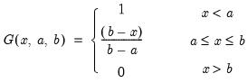
Uniform cumulative distribution.
Syntax: @cunif(x, a, b[, u])
x: number
a: number
b: number,

u: (optional) number
Return: number
Computes the cumulative distribution function
If the optional argument u is non-zero, return the upper-tail value:
Examples
= @cunif(4, 1, 6)
returns 0.6.
Cross-references
See also
@dunif,
@qunif, and
@runif.
Count of matching values in each column.
Syntax: @cvalcount(x, y)
x: data object
y: value or string
Return: vector
The number of elements in each column of x that match y. Note that numeric matches require an exact match.
Examples
Let X be a matrix. Then
= @cvalcount(x, 2)
returns a vector containing the number of elements in each column of X that take the value 2.
Cross-references
Variance (population) of each column of a matrix.
Syntax: @cvar(m)
m: matrix
Return: vector
Returns the column population variance.
Examples
= @cvar(mat)
returns a (column) vector whose i-th element is the population variance for the i-th column of MAT.
Cross-references
Variance (population) of each column of a matrix.
Syntax: @cvarp(m)
m: matrix
Return: vector
Returns the column population variance.
Examples
= @cvarp(mat)
returns a (column) vector whose i-th element is the population variance for the i-th column of MAT.
Cross-references
Variance (sample) of each column of a matrix.
Syntax: @cvars(m)
m: matrix
Return: vector
Returns the column sample variance.
Examples
= @cvars(mat)
returns a (column) vector whose i-th element is the sample variance for the i-th column of MAT.
Cross-references
Weibull cumulative distribution.
Syntax: @cweib(x, m, a[, u])
x: number,

m: number,

a: number,

u: (optional) number
Return: number
Computes the cumulative distribution function
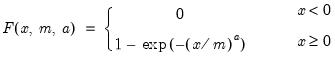 | (18.4) |
If the optional argument u is non-zero, return the upper-tail value:
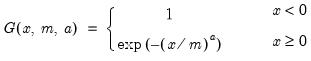 | (18.5) |
Examples
= @cweib(@log(2), 1, 1)
returns 0.5.
Cross-references
See also
@dweib,
@qweib, and
@rweib.