Function Reference: D
d Difference (time-series) functions for series.
@date Date number of observation.
@dateadd Date number after applying offset.
@datediff Difference between two date numbers.
@dateceil Last possible date in a time period.
@datefloor Earliest possible date in a time period.
@datenext First possible date in the next time period.
@datestr String representation of a date number.
@dateval Date number associated with a string representation of a date.
@daycount Number of days of week in observation.
@dbeta Beta distribution probability density.
@dbinom Binomial probability function.
@dbname String containing the default database name.
@dbvnorm Bivariate normal probability density function.
@dchisq Chi-square probability density function.
@dcumdn Difference of cumulative sum of negative (below threshold) changes in a series.
@dcumdp Difference of cumulative sum of positive (above threshold) changes in a series.
@dcumdz Difference of cumulative sum of zero (at threshold) changes in a series.
@demean Compute deviations from the mean of the series.
@demeanby Compute deviations from the mean of the series by group.
@det Determinant of matrix.
@detrend Compute deviations from the trend of the series.
@dexp Exponential probability density function.
@dextreme Extreme value (Type I-minimum) distribution function.
@dfdist F-distribution probability density function.
@dgamma Gamma probability density function.
@dged Generalized error probability density function.
@digamma First derivative of the natural log gamma function.
@diwish Inverse Wishart probability density function.
@dlaplace Laplace probability density function.
dlog Difference functions for natural logarithm of a series.
@dlognorm Log normal probability density function.
@dmvnorm Multivariate normal probability density function.
@dnegbin Negative binomial probability function.
@dnorm Standard normal probability density function.
@dpareto Pareto probability density function.
@dtdist Student’s

probability density function.
@dtoo Observation number in the workfile associated with a date string.
@dunif Uniform probability density function.
@dupselem Identifier for the observation within the set of duplicates.
@dupsid Identifier for the duplicates group for the observation.
@dupsobs Number of observations in the corresponding duplicates group.
@during Indicator of whether an observation is between two dates.
@dweib Weibull probability density function.
@dwish Wishart probably density function.
Difference (time-series) functions for series.
• First difference function for series.
Syntax: d(x)
x: series
Return: series
Computes
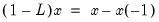
where

is the lag operator.
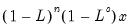
• n-th order difference function for series.
Syntax: d(x, n)
x: series
n: integer, series
Return: series
Computes

where

is the lag operator.
If
n is not an integer, the integer floor

will be used.
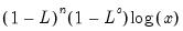
• n-th order difference function for series with an s-th seasonal difference.
Syntax: d(x, n, s)
x: series
n: integer
s: integer
Return: series
Computes
where

is the lag operator.
If
n or
s are not integers, the integer floors

and

will be used.
These functions are panel aware.
Examples
The code below produces a graph of a random walk process and its first difference:
wfcreate u 1000
series y = 0
smpl @first+1 @last
series y = y(-1) + nrnd
smpl @all
group g y d(y)
g.line
The first line creates an unstructured workfile containing a thousand observations. Lines two through five create the series y containing the realization of a random walk process initialized at 0. Lines six and seven graphs y and d(y) together.
Cross-references
Path of the current EViews data directory.
Syntax: @datapath
Return: string
Returns a string containing the location of the current EViews data directory.
Examples
If your current working directory is d:\data
%y = @datapath
assigns a string of the form “D:\DATA”.
Cross-references
Date number of observation.
Syntax: @date
Return: series
Returns the date number associated with each observation in the workfile.
The date number associated with an observation is the first (smallest) date number corresponding to the observation date interval.
Examples
series dt = @date
saves the date numbers into the series DT. The default display format for these numbers will match the workfile frequency, but you may work with and display the series values as numbers.
alpha dts_1 = @datestr(@date,"yyyy:q")
alpha dts_2 = @strdate("yyyy:q")
Create two string series with the observation dates formatted in “yyyy:q” format.
Cross-references
Date number after applying offset.
Syntax: @dateadd(d, offset, u[, f])
d: date number, series, vector
offset: integer, series, vector
u: time unit string
f: (optional) number
Return: date number, series, vector
Returns the date number given by d offset by offset time units as specified by the time unit string u. The optional parameter f controls handling of business days.
• The valid time unit string values are: “A” or “Y” (annual), “S” (semi-annual), “Q” (quarters), “MM” (months), “WW” (weeks), “DD” (days), “B” (business days), “HH” (hours), “MI” (minutes), “SS” (seconds).
• When the time unit u is business days (“B”), the optional control flag parameter f controls how a non-business day date number d is handled. When f is absent or equal to zero, the date number d is automatically advanced to the next business day before offset is applied. Otherwise, when f is non-zero automatic advancement is suppressed. Consequently, when f is non-zero and offset is 0 the function returns the original date number d (a non-business day).
Examples
Suppose that the value of d is 730088.0 (midnight, December 1, 1999).
Then we can add and subtract 10 days from the date by using the functions
@dateadd(730088.0, 10, "dd")
@dateadd(730088.0, -10, "dd")
which return 730098.0 (December 11, 1999) and (730078.0) (November 21, 1999). Note that these results could have been obtained by taking the original numeric value plus or minus 10.
To add 5 weeks to the existing date, simply specify “WW” as the time unit string:
@dateadd(730088.0, 5, "ww")
returns 730123.0 (January 5, 2000).
To find the date 3 months prior to the existing date, specify “MM” as the time unit string:
@dateadd(730088.0, -3, "mm")
The function may usefully be combined with other date functions. To find the day of the week 4 months from DD:
@datestr(@dateadd(dd, 4, "mm"), "Wdy")
Business day adjustments are slightly more complex. Suppose that the value of DD is 730091.0 (midnight, December 4, 1999), which is a Saturday:
730091.0
Then the previous business day, may be obtained by
@dateadd(dd, -1, "b")
@dateadd(dd, -1, "b", 1)
which both return 730090.0 (December 3, 1999), the preceding Friday.
A business day offset of 0 with a zero (or omitted) control flag f, automatically advances to the next business day
@dateadd(dd, 0, "b")
returns 730093.0 (December 6, 1999), the following Monday.
A business day offset of 0 with a non-zero control flag f, does not advance from the original day, so that
@dateadd(dd, 0, "b", 1)
returns 730091.0 (December 4, 1999), the original Saturday.
Automatic business day adjustments are performed prior to applying the offset parameter, so that
@dateadd(dd, 1, "b")
returns 730094.0 (December 7, 1999), the following Tuesday, while
@dateadd(dd, 1, "b", 1)
returns 730093.0 (December 6, 1999), the following Monday.
If DSER is a series containing date numbers,
series dser1 = @dateadd(dser, 3, "mm")
produces the 3-month date number offsets associated for each observation for DSER in the workfile sample. You may use “@date” in place of DSER to obtain results using the built-in dates in the workfile structure.
If DVEC is an vector containing date numbers,
vector avec = @dateadd(dvec, 3, "mm")
produces the 3-month date number offsets for elements of the vector.
Cross-references
See
“Dates” and
“Date Formats” for additional details on date numbers and date format strings.
Difference between two date numbers.
Syntax: @datediff(d1, d2, u[, f])
d1: date number, series, vector
d2: date number, series, vector
u: time unit string
f: (optional) number
Return: date number, series, vector
Returns the difference between two date numbers d1 and d2, measured by time units specified by the time unit string u. The optional parameter f controls handling of business days.
• The valid time unit string values are: “A” or “Y” (annual), “S” (semi-annual), “Q” (quarters), “MM” (months), “WW” (weeks), “DD” (days), “B” (business days), “HH” (hours), “MI” (minutes), “SS” (seconds).
• When the time unit u is business days (“B”), the optional control flag parameter f controls how a non-business day date number d is handled. When f is absent or equal to zero, the date number d is automatically advanced to the next business day before offset is applied. Otherwise, when f is non-zero automatic advancement is suppressed. Consequently, when f is non-zero and offset is 0 the function returns the original date number d (a non-business day).
Examples
Suppose d1 is 730088.0 (December 1, 1999) and d2 is 729754.0 (January 1, 1999). We may define
scalar d1 = 730088.0
scalar d2 = 729754.0
The two commands
@datediff(730088.0, 729754.0, "dd")
@datediff(d1, d2, "dd")
return 334 for the number of days between the two dates. Note that this is result is simply the difference between the two numbers.
The following expressions calculate differences in months and weeks:
@datediff(730088.0, 729754.0, "mm")
@datediff(730088.0, 729754.0, "ww")
and
@datediff(d1, d2, "mm")
@datediff(d1, d2, "22")
return 11 and 47 for the number of months and weeks between the dates.
Business day computations are slightly more complex. Suppose that d1 is 730094.0 (midnight, December 7, 1999), which is a Tuesday, and d2 is 730091.0 (midnight, December 4, 1999), which is the preceding Saturday:
scalar d1 = 730094.0
scalar d2 = 730091.0
@datediff(d1, d2, "b")
returns 1 for the number of business days between the two dates since the absence of the control flag means that the d2 date automatically advances to the next business day
@datediff(d1, d2, "b", 1)
returns 2 for the number of business days between the two dates since, control flag argument of 1 means that the d2 date does not automatically advance to the next (Monday) business day.
If DSER1 and DSER2 are series containing date numbers,
series dser3 = @datediff(dser1, ders2, "mm")
compute the month differences for each observation for DSER1 and DSER2 in the workfile sample.
If DVEC1 and DVEC2 are vectors containing date numbers,
vector dvecdiff = @datediff(dvec1, dvec2, "mm")
compute the month differences for all elements of the vectors.
Cross-references
See
“Dates” and
“Date Formats” for additional details on date numbers and date format strings.
Last possible date in a time period.
Syntax: @dateceil(d, u[, step])
d: date number, series, vector
u: time unit string
step: (optional) integer, series, vector
Return: date number, series, vector
Finds the last possible date number associated with d in the regular frequency defined by the given time unit u and optional step integer step. The regular frequency is defined relative to the basedate of midnight, January 2001.
• The valid time unit string values are: “A” or “Y” (annual), “S” (semi-annual), “Q” (quarters), “MM” (months), “WW” (weeks), “DD” (days), “B” (business days), “HH” (hours), “MI” (minutes), “SS” (seconds).
• If step is omitted, the frequency will use a step of 1, so that by default, @dateceil will find the end of the period defined by the time unit.
Examples
Suppose that d is 730110.8 (7 PM, December 23, 1999).
Then the command
@dateceil(730110.8, "dd")
gives the last date number associated with the end of December 23, 1999, yielding 730110.999 (11:59:59.999... PM, December 23, 1999).
Similarly, the command,
@dateceil(730110.8, "mm")
gives the date number associated with the end of month of December 1999 (11:59:59.999... PM, December 31, 1999) giving 730118.999.
The commands
@dateceil(730110.8, "hh", 3)
@dateceil(730110.8, "hh", 6)
return 730110.874999 (8:59:59.999... PM, December 23, 1999), and 730110.999 (11:59:59.999... PM, December 23, 1999), which are the last date numbers for 3 and 6 hour regular frequencies anchored at midnight, January 1, 2001.
If DSER is a series containing date numbers,
series dser1 = @dateceil(dser, "mm")
gives the date number of the end of the month for each observation in DSER in the workfile sample. You may use “@date” in place of DSER to obtain results using the built-in dates in the workfile structure.
If DVEC is a vector containing date numbers,
vector avec = @dateceil(dvec, "y")
gives the last date number in the year for each element of the vector.
Cross-references
See
“Dates” and
“Date Formats”for additional details on date numbers and date format strings.
First possible date in a time period.
Syntax: @datefloor(d, u[, step])
d: date number, series, vector
u: time unit string
step: (optional) integer, series, vector
Return: date number, series, vector
Finds the first possible date number associated with d in the regular frequency defined by the given time unit u and optional step integer step. The regular frequency is defined relative to the basedate of midnight, January 2001.
• The valid time unit string values are: “A” or “Y” (annual), “S” (semi-annual), “Q” (quarters), “MM” (months), “WW” (weeks), “DD” (days), “B” (business days), “HH” (hours), “MI” (minutes), “SS” (seconds).
• If step is omitted, the frequency will use a step of 1, so that by default, @dateceil will find the end of the period defined by the time unit.
Examples
Suppose that d is 730110.8 (7 PM, December 23, 1999).
Then the command
@datefloor(730110.8, "dd")
gives the first date number associated with the end of December 23, 1999, yielding 730110.0 (midnight, December 23, 1999).
Similarly, the command
@datefloor(730110.8, "mm")
returns 730088.0 (midnight, December 1, 1999), the date number for the beginning of the associated with 730110.8.
The commands
@datefloor(730110.8, "hh", 6)
@datefloor(730110.8, "hh", 12)
return 730110.75 (6 PM, December 23, 1999), and 730110.5 (Noon, December 23, 1999), which are the earliest date numbers for 6 and 12 hour regular frequencies anchored at Midnight, January 1, 2001.
If DSER is a series containing date numbers,
series dser1 = @datefloor(dser, "mm")
gives the date number of the beginning of the month for each observation in DSER in the workfile sample. You may use “@date” in place of DSER to obtain results using the built-in dates in the workfile structure.
If DVEC is a vector containing date numbers,
vector avec = @datefloor(dvec, "y")
gives the first date number in the year for each element of the vector.
Cross-references
See
“Dates” and
“Date Formats”for additional details on date numbers and date format strings.
First possible date in next time period.
Syntax: @datenext(d, u[, step])
d: date number, series, vector
u: time unit string
step: (optional) integer, series, vector
Return: date number, series, vector
Finds the first possible date number in the next regular frequency period following d, defined by the given time unit u and optional step integer step. The regular frequency is defined relative to the basedate of midnight, January 2001.
• The valid time unit string values are: “A” or “Y” (annual), “S” (semi-annual), “Q” (quarters), “MM” (months), “WW” (weeks), “DD” (days), “B” (business days), “HH” (hours), “MI” (minutes), “SS” (seconds).
• If step is omitted, the frequency will use a step of 1, so that by default, @datenext will find the end of the period defined by the time unit.
Examples
Suppose that date1 is 730110.8 (7 PM, December 23, 1999).
Then the commands
@datenext(730110.8, "dd")
@datenext(730110.8, "mm")
yield 730111.0 (midnight, December 24, 1999) and 730119.0 (midnight, January 1, 2000), the date numbers for the beginning of the day and month following the date number 730110.8, respectively.
Similarly,
@datenext(730110.8, "hh", 3)
@datenext(730110.8, "hh", 6)
return 730110.875 (9 PM, December 23, 1999), and 730111 (midnight, December 24, 1999), which are the earliest date numbers for the subsequent 3 and 6 hour regular frequencies anchored at midnight, January 1, 2001.
If DSER is a series containing date numbers from the workfile structure
series dser1 = @datenext(dser, "mm")
gives the date number of the beginning of the next month for each observation in DSER in the workfile sample. You may use “@date” in place of DSER to obtain results using the built-in dates in the workfile structure.
If DVEC is a vector containing date numbers,
vector avec = @datenext(dvec, "y")
gives the first date number in the next year for each element of the vector.
Cross-references
Extract part of a date number.
Syntax: @datepart(d, fmt)
d: date number, series, vector
fmt: date format string
Return: number, series, vector
Returns a number representing part of a date, using a date number corresponding to the date and a fmt, where fmt is a component of a date format string.
Examples
Consider the d date number value 730110.5 (noon, December 23, 1999).
The values for
@datepart(730110.5, "dd")
@datepart(730110.5, "w")
@datepart(730110.5, "ww")
@datepart(730110.5, "mm")
@datepart(730110.5, "yy")
are 23 (day of the month), 1 (day of the week), 52 (week in the year), 12 (month in the year), and 99 (year), respectively).
If DSER is a series containing date numbers,
series dser1 = @datepart(dser, "mm")
gives the month of the year given by each observation in DSER in the workfile sample. You may use “@date” in place of DSER to obtain results using the built-in dates in the workfile structure.
If AVEC is a vector containing date numbers,
vector avec1 = @datenext(avec, "y")
returns the year for each element of the vector.
Cross-references
See
“Dates” and
“Date Formats”for additional details on date numbers and date format strings.
String representation of a date number.
Syntax: @datestr(d[, fmt])
d: date number, series, vector
fmt: (optional) date format string
Return: string, alpha, svector
Convert the numeric date value,
d, into a string representation of a date using the optional format string
fmt. Date format syntax is outlined in
“Date Formats”.
If a fmt is not provided, EViews will use the global default settings for the to determine the ordering of days and months in the string.
Next, EViews examines the date values to be translated and looks for relevant time-of-day information. If there is relevant time-of-day information, EViews will extend the date format accordingly by adding relevant hours, minutes, and seconds information, in that order. Thus, if days are favored in the global default ordering, and relevant hours (but not minutes and seconds) information is present, EViews will use
"dd/mm/yyyy hh"
while if hours-minutes are present, the default format will be
"dd/mm/yyyy hh:mi"
and so forth.
Examples
Consider the d date number value 730088 (midnight, December 1, 1999).
Then
@datestr(730088, "mm/dd/yy")
will return “12/1/99”,
@datestr(730088, "DD/mm/yyyy")
will return “01/12/1999”, and
@datestr(730088, "Month dd, yyyy")
will return “December 1, 1999”, and
@datestr(730088, "w")
will produce the string “3”, representing the weekday number for December 1, 1999.
You may use text to delimit the date format components,
@datestr(730088, "yyyy:q")
@datestr(730088, "yyyy[q]q")
produces “1999:4” and “1999q4”. Note the use of the square brackets to pass through the literal “q” string to the string output. If the workfile is quarterly, then
@datestr(730088, "yyyy[q]q")
also returns “1999q4” as the “f” will return the frequency delimiter from the active workfile page.
If DSER is a series containing date numbers,
alpha aser1 = @datestr(dser, "Month dd, yyyy")
produces the formatted date string for each observation in DSER in the workfile sample.
If DVEC is a vector containing date numbers,
svector avec = @datestr(dvec, "DD/mm/yyyy")
returns a svector containing strings with the day, month, and year, corresponding to each element of the DVEC vector.
Cross-references
See
“Dates” and
“Date Formats” for additional details on date numbers and date format strings.
See
@strdate to obtain workfile date strings. See also
@dateval for converting date strings to date numbers.
Convert the string representation of a date into a date number.
Syntax: @dateval(str1[, fmt])
str1: string, alpha, svector
fmt: (optional) date format string
Return: date number, series, vector
Returns the date number associated with the string representation of a date, str. Interpretation of the string may be controlled of using the optional format string fmt.
Examples
@dateval("12/1/1999", "mm/dd/yyyy")
contains the date number (730088) for December 1, 1999. The format indicates that the string represents a one or two-digit month identifier, a “/” separator, a one or two-digit day identifier, a “/” separator, and a 4-digit year identifier.
@dateval("12/1/1999", "dd/mm/yyyy")
contains the date number (729765) for January 12, 1999. The format reverses the month and day identifiers used above.
If ALPHA1 is an alpha series, the command
series ser1 = @dateval(alpha1, "yyyy-MM-DD HH:mi:ss")
fills DSER with date numbers associated with the ISO 8601 representation of the string dates for each observation in the workfile sample. Here, we have used the capitalized forms of “MM”, “DD”, and “HH” to ensure that we interpret the required leading zeros.
If AVEC1 is an svector, the commands
svector vec1 = @dateval(avec1, "yyyy-Month-dd")
fills DVEC with the date numbers associated with the strings in AVEC1, interpreted as a four-digit year, followed by the full name of the month (with first letter capitalized), and the one or two-digit day identifier, all separated by dashes.
Cross-references
See
“Dates” and
“Date Formats”for additional details on date numbers and date format strings.
See
@datestr for converting date numbers to date strings, and
@strdate for obtaining strings for workfile dates.
Day of observation.
Syntax: @day
Return: series
Returns the day of the month (1-31) associated with each observation in the workfile.
• If the workfile is of lower than daily frequency, all observations will be set to 1.
• If the workfile is undated, observations will be set to -1.
Examples
series dt = @day
saves the days of the month into the series DT.
The command
smpl if @day > 29
sets the sample to only use days 30 and 31 of months.
Cross-references
Number of calendar days in observation.
Syntax: @daycount(d)
d: string, alpha
Return: series
Returns the number of calendar days within each observation of the workfile.
The optional d argument lets you specify an individual day or range of days of the week to count (e.g., “Mon”, “Tues-Thurs”, or “Fri Sat”).
• If only one weekday is provided, @daycount returns the number of times that particular weekday occurs within the observation.
• If two weekdays are provided, @daycount returns the number of times that any weekday between the two weekdays (inclusive) occurs within the observation.
If the workfile is undated, the function with return NAs.
Examples
series modays = @daycount("Mon")
creates a series with the number of Mondays in each observation.
series wkdays = @daycount(Mon Fri)
fills WKDAYS with the number of weekdays, while
series wenddays = @daycount("Sat Sun")
counts the number of weekend days in each observation.
workfile m 2020 2022
smpl if @daycount("Sat") > 4
creates a monthly workfile, and sets the sample to those months with 5 Saturdays.
Cross-references
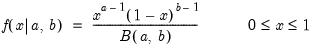
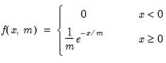
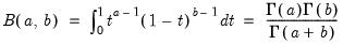
Beta distribution probability density.
Syntax: @dbeta(x, a, b)
x: number
a: number,

b: number,

Return: number
Evaluates the probability density function,
and 0 elsewhere, where

is the beta function
Examples
= @dbeta(0.5, 1, 2)
returns 1.
Cross-references
See also
@cbeta,
@qbeta, and
@rbeta.
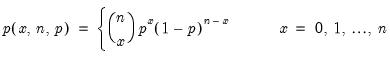
Binomial distribution probability.
Syntax: @dbinom(x, n, p)
x: number
n: integer,

p: number,

Return: number
Evaluates the probability function,
and 0 elsewhere.
Examples
= @dbinom(2, 5, 0.5)
returns 0.3125.
Cross-references
Default database name.
Syntax: @dbname
Return: string
Returns a string containing the name of the current default database.
Examples
string dbname = @dbname
creates a string variable with the default database name.
Cross-references
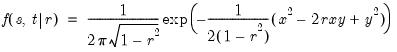
Bivariate normal probability density.
Syntax: @dbvnorm(x, y, r)
x: number
y: number
p: number,

Return: number
Computes the bivariate normal density with 0 mean, unit variances, and correlation r:
Examples
= @dbvnorm(0, 0, 0.5)
returns 0.18377....
Cross-references
Chi-square probability density.
Syntax: @dchisq(x, v)
x: number
v: number,

Return: number
Evaluates the probability density function,
for

or 0 elsewhere.
Examples
= @dchisq(100, 100)
returns 0.02816....
Cross-references
Difference of the cumulative process of negative (below threshold) changes.
Compute the difference of the partial sum process of negative (below the threshold y) changes in the series x beginning in the specified date.
Syntax: @dcumdn(x, d[, y, s])
x: series
d: string
y: (optional) number
s: (optional) sample string or object
Return: series
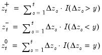
Consider the partial sum decomposition of a variable

given a initial value

as

where

,

, and

are the partial sum processes of the differences for positive, negative, and zero
changes in

relative to the threshold
y:
The function returns the negative accumulation
for the current or specified sample.
• The date
d string specification determines

.
• Values for dates prior to d will be NAs.
• The optional

argument specifies the threshold value. By default

.
This function is panel aware.
Examples
The code below produces a graph of @cumdn and @dcumdn applied on the sine wave x.
wfcreate u 50
series x = @sin(@pi*@trend/4)
group g @cumdn(x,1) @dcumdn(x,1)
g.line
Cross-references
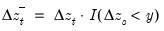
Difference of the cumulative process of positive (above threshold) changes.
Compute the difference of the partial sum process of positive (above the threshold y) changes in the series x beginning in the specified date.
Syntax: @dcumdp(x, d[, y, s])
x: series
d: string
y: (optional) number
s: (optional) sample string or object
Return: series
Consider the partial sum decomposition of a variable

given a initial value

as

where

,

, and

are the partial sum processes of the differences for positive, negative, and zero
changes in

relative to the threshold
y:
The function returns the positive accumulation
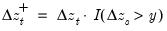
for the current or specified sample.
• The date
d string specification determines

.
• Values for dates prior to d will be NAs.
• The optional

argument specifies the threshold value. By default

.
This function is panel aware.
Examples
The code below produces a graph of @cumdp and @dcumdp applied on the sine wave x.
wfcreate u 50
series x = @sin(@pi*@trend/4)
group g @cumdp(x,1) @dcumdp(x,1)
g.line
Cross-references
Difference of the cumulative process of zero (at threshold) changes.
Compute the difference of the partial sum process of zero (at the threshold y) changes in the series x beginning in the specified date.
Syntax: @dcumdz(x, d[, y, s])
x: series
d: string
y: (optional) number
s: (optional) sample string or object
Return: series
Consider the partial sum decomposition of a variable

given a initial value

as
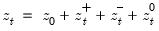
where

,

, and

are the partial sum processes of the differences for positive, negative, and zero
changes in

relative to the threshold
y:
The function returns the zero accumulation
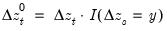
for the current or specified sample.
• The date
d string specification determines

.
• Values for dates prior to d will be NAs.
• The optional

argument specifies the threshold value. By default

.
This function is panel aware.
Examples
show @dcumdz(x, 2001, 1)
produces a linked series of @dcumdz applied to x where the starting date is 2001 and the threshold value is set to 1.
Cross-references
Compute deviations from the mean of the series.
Syntax: @demean(x[, s])
x: series, vector, matrix
s: (optional) sample string or object when x is a series and assigning result to a series
Return: series, vector, matrix
Returns a copy of x after subtracting off the mean.
For series calculations, EViews will use the current or specified workfile sample.
This function is panel aware.
Examples
The code below produces a graph of a series and its demeaned form:
wfcreate m 2000 2020
series y = 10 + nrnd
group g y @demean(y)
g.line
The first line creates a monthly workfile starting in January 2000 and ending in December 2020. The second line generates a series y equal to 10 plus normal error. The last two lines graphs y and @demean(y) together.
Cross-references
Compute deviations of the mean of series by group.
Syntax: @demeanby(x, g[, s])
x: series
g: series
s: (optional) sample string or object
Return: series
Returns a copy of x after subtracting off group means, where groups are defined by the series or vector g.
EViews will use the current or specified workfile sample.
This function is panel aware.
Examples
The code below produces a graph of a series and its demeaned-by-group form:
wfcreate m 2000 2020
series y = @month + nrnd
group g y @demeanby(y, @month)
g.line
The first line creates a monthly workfile starting in January 2000 and ending in December 2020. The second line generates a series y equal to the month of the year plus normal error. The last two lines graphs y and @demeanby(y, @month) together.
Cross-references
See also
@demean and
@detrend.
Determinant of matrix.
Syntax: @det(m)
m: matrix, sym
Return: number
Calculate the determinant of the square matrix or sym, m.
The determinant is nonzero for a nonsingular matrix and 0 for a singular matrix.
Examples
matrix m1 = @mnrnd(4, 4)
scalar sc1 = @det(m1)
computes the determinant of the matrix M1.
sym s1 = @inner(m1)
= @det(s1)
returns the determinant of the symmetric matrix S1.
Cross-references
Compute deviations from the trend of a series.
Syntax: @detrend(x[, s])
x: series, vector, matrix
s: (optional) sample string or object when x is a series and assigning result to a series
Return: series, vector, matrix
Returns the residuals of an OLS regression of the data versus an intercept and an implicit time trend.
For series calculations, EViews will use the current or specified workfile sample.
This function is panel aware.
Examples
The code below produces a graph of a series and its detrended form:
wfcreate m 2000 2020
series y = @trend + nrnd
group g y @detrend(y)
g.line
The first line creates a monthly workfile starting in January 2000 and ending in December 2020. The second line generates a series y equal to trend plus normal error. The last two lines graphs y and @detrend(y) together.
Cross-references
Exponential probability density.
Syntax: @dexp(x, m)
x: number
m: number,

Return: number
Evaluates the probability density function,
Examples
= @dexp(@log(2), 1)
returns 0.5.
Cross-references
See also
@cexp,
@qexp, and
@rexp.
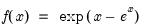
Extreme value (Type I-minimum) probability density.
Syntax: @dextreme(x)
x: number
Return: number
Evaluates the probability density function,
Examples
= @dextreme(1)
returns 0.17937....
Cross-references
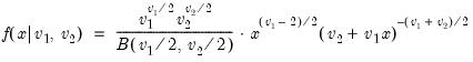
F-distribution probability density.
Syntax:
@dfdist(
x,  ,
,  )
) x: number

: number,


: number,

Return: number
Evaluates the probability density function,
for

and 0 otherwise, where

is the beta function
Note that the functions allow for fractional degrees of freedom parameters

and

.
Examples
= @dfdist(1, 2, 2)
returns 0.25.
Cross-references
Gamma probability density.
Syntax: @dgamma(x, b, r)
x: number
b: number,

r: number,

Return: number
Evaluates the probability density function,
for

and 0 elsewhere.
Examples
= @dgamma(2, 4, 1)
returns 0.15163....
Cross-references
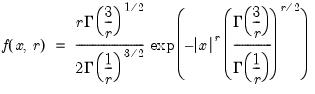
Generalized error probability density.
Syntax: @dged(x, v)
x: number
r: number,

Return: number
Evaluates the probability density function,
Examples
= @dged(0, 2)
returns 0.39894....
Cross-references
See also
@cged,
@qged, and
@rged.
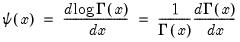
First derivative of the natural log gamma function.
Syntax: @digamma(x)
x: number
Return: number
Computes the derivative of the log of the gamma function:
for  .
. Examples
= @digamma(1)
returns -0.57721....
Cross-references
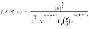
Inverse Wishart probability density.
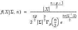
Syntax: @diwish(X, S, n)
@diwishc(X, S, n)
@diwishi(X, S, n)
@diwishic(X, S, n)
X: sym,

S: sym, matrix,

n: number,

Return: number
Evaluate the inverse Wishart distribution

density function for sym values of
X, and

.
The inverse Wishart density is given by
where

and

are symmetric

matrices, and

.
There are four different forms of the density evaluation function, corresponding to different ways of specifying

. The forms are distinguished by different suffixes that are applied to the base “@dwish” command and how they change the interpretation of the
S matrix argument:
@diwish | “” | Supply  . |
@diwishc | “c” | Supply the Cholesky decomposition of  . This form is more efficient when performing multiple draws from the same distribution (compute the Cholesky once, but sample many times). |
@diwishi | “i” | Supply  . This form is more efficient than explicitly inverting  to supply  . |
@diwishic | “ic” | Supply the Cholesky decomposition of  . This form combines the efficiencies of the Cholesky and inverse forms. |
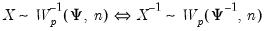
Note that if

is an inverse Wishart random variable, then

follows a Wishart distribution:
Examples
= @diwish(@identity(3), @identity(3), 5)
returns 0.00018....
Cross-references
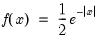
Laplace probability density.
Syntax: @dlaplace(x)
x: number
Return: number
Evaluates the probability density function,
Examples
Cross-references
= @dlaplace(@log(2))
returns 0.25.
Difference functions for natural logarithm of series.
• First difference function for natural logarithm of the series.
Syntax: dlog(x)
x: series
Computes

where

is the lag operator.
• n-th order difference function for natural logarithm of series.
Syntax: dlog(x, n)
x: series
n: integer, series
Return: series
Computes 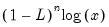
for integer

where

is the lag operator.
If
n is not an integer, the integer floor

will be used.
• n-th order difference function for natural logarithm of series with an s-th seasonal difference.
Syntax: dlog(x, n, s)
x: series
n: integer, series
s: integer, series
Return: series
Computes
for integer

where

is the lag operator.
If
n or
s are not integers, the integer floors

and

will be used.
These functions are panel aware.
Examples
show dlog(y,2)
is equivalent to d(log(y),2), the 2nd-order difference of the log of the series y.
Cross-references
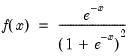
Logistic probability density.
Syntax: @dlogistic(x)
x: number
Return: number
Evaluates the probability density function,
Examples
= @dlogistic(0)
returns 0.25.
Cross-references
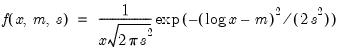
Log normal probability density.
Syntax: @dged(x, m, s)
x: number
m: number,

s: number,

Return: number
Evaluates the probability density function,
for

and 0 otherwise.
Examples
= @dlognorm(1, 0, 2)
returns 0.19947....
Cross-references
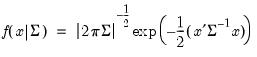
Multivariate normal probability density.
Syntax: @dmvnorm(x, S)
@dmvnormc(x, S)
@dmvnormi(x, S)
@dmvnormic(x, S)
x: vector
S: sym, matrix
Return: number
Evaluate the multivariate normal

density function for vector values of
x, and sym

.
The mean zero multivariate normal density is given by
There are four different forms of the density evaluation function, corresponding to different ways of specifying

. The forms are distinguished by different suffixes that are applied to the base “@dmvnorm” command and how they change the interpretation of the
S matrix argument:
@dmvnorm | “” | Supply  . |
@dmvnormc | “c” | Supply the Cholesky decomposition of  . This form is more efficient when performing multiple draws from the same distribution (compute the Cholesky once, but sample many times). |
@dmvnormi | “i” | Supply  . This form is more efficient than explicitly inverting  to supply  . |
@dmvnormic | “ic” | Supply the Cholesky decomposition of  . This form combines the efficiencies of the Cholesky and inverse forms. |
Examples
= @dmvnorm(@zeros(3), @identity(3))
returns 0.06349....
Cross-references
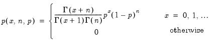
Negative binomial distribution probability.
Syntax: @dnegbin(x, n, p)
x: number
n: number,

p: number,

Return: number
Evaluates the probability function,
Examples
= @dnegbin(9, 10, 0.5)
returns 0.09273....
Cross-references
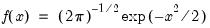
Standard normal probability density.
Syntax: @dnorm(x)
x: number
Return: number
Evaluates the probability density function,
Examples
= @dnorm(0)
returns 0.39894....
Cross-references
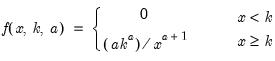
Pareto probability density.
Syntax: @dpareto(x, k, a)
x: number
k: number,

a: number,

Return: number
Evaluates the probability density function,
Examples
= @dpareto(2, 1, 2)
returns 0.25.
Cross-references
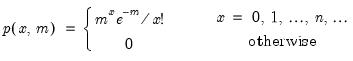
Poisson distribution probability.
Syntax: @dpoisson(x, m)
x: number
m: number,

Return: number
Evaluates the probability function,
Examples
= @dpoisson(10, 10)
returns 0.12511....
Cross-references
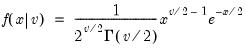
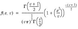
Student’s

probability density.
Syntax: @dtdist(x, v)
x: number
v: number
Return: number
Evaluates the probability density function,
for  , and
, and 
Examples
= @dtdist(0, 1)
returns 0.31830....
Cross-references
Date-to-(workfile) observation.
Syntax: @dtoo(str)
str: string, alpha, svector
Return: integer, series, vector
Returns the observation number corresponding to the workfile date contained in the string. The observation number is relative to the start of the current workfile range, not the current sample.
Note that EViews will use the global default settings for the to determine the ordering of days and months in the string.
@dtoo will generate an error if used in a panel structured workfile.
Examples
Suppose that the workfile contains quarterly data from 1990q1 to 2020q4. Consider the commands
scalar obsnum = @dtoo("1994m01")
scalar gdpval1 = gdp(obsnum + 10)
scalar gdpval2 = gdp(@dtoo("1994m01") + 10)
The first line returns 17, the observation in the workfile corresponding to 1990q1, and the latter two find the value of GDP in 1996q3. Note that since we are assigning the value to a scalar on the left, the argument in GDP is interpreted as an element, not a lag.
The command
series dser = @dtoo("12/1/1999")
fills DSER with the observation number corresponding to “12/1/1999” for each observation in the workfile sample, where the months and days are interpreted using the global settings.
If the alpha series ASER contains dates,
series dser = @dtoo(aser)
fills DSER with the observation number corresponding to the string dates in ASER for each observation in the workfile sample.
If AVEC is an svector, the command
vector dvec = @dtoo(avec)
fills DVEC with the observation numbers associated with the strings in AVEC.
Cross-references
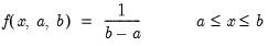
Uniform probability density.
Syntax: @dunif(x, a, b)
x: number
a: number
b: number,

Return: number
Evaluates the probability density function,
and 0 otherwise.
Examples
= @dunif(4, 1, 6)
returns 0.2.
Cross-references
See also
@cunif,
@qunif, and
@runif.
Duplication matrix.
Syntax: @duplic(n)
n: integer
Return: matrix
The duplication matrix transforms the half vectorization of a sym matrix to the full vectorization of the matrix.
Given the

sym matrix

, returns the
matrix

, which satisfies
Examples
sym s1 = @unvech(@mnrnd(15))
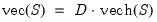
vector diff = @vec(s1) - @duplic(s1.@cols) * @vech(s1)
demonstrates the properties of the duplication matrix since DIFF equals zero.
Cross-references
Inverse duplication matrix.
Syntax: @duplicinv(n)
n: integer
Return: matrix
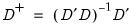
The inverse of the duplication matrix transforms the vectorization of a sym matrix to the half vectorization of the matrix.
Returns

, the
Moore-Penrose inverse of the duplication matrix where
for

, the duplication matrix satisfying
for an

symmetric matrix

, so that
Examples
The commands
sym s2 = @unvech(@mnrnd(15))
vector diff = @duplicinv(s2.@cols) * @vec(s2) - @vech(s2)
demonstrates the properties of the inverse duplication matrix since DIFF equals zero.
Cross-references
Duplicate identifier within group.
Identifier for the observation within the duplicate group, enumerating observations with the same values.
Syntax: @dupselem(x1,[x2, x3, ... ], [s])
x: series, alpha, group, vector, matrix
x#: series, alpha, group, vector, matrix
s: (optional) sample string or object when the x are series, alpha, and groups and assigning to series
Return: series, vector
For series, alpha, and groups, a duplicate is defined as two observations having identical values for all of variables given by the arguments.
For vectors and matrix objects, a duplicate is defined as two row identifiers having identical values in each of the vector and matrix objects given by the arguments.
Once sets of duplicates are identified, the observations or rows within each set are enumerated. For a set consisting of n duplicated values, the enumerated values are simply the integer values from 1 to n.
Examples
Let X be a series of length 10 that alternates between 0 and 1. Then
show @dupselem(x)
will display a series whose observations are 1, 1, 2, 2, 3, 3, 4, 4, 5, 5, which enumerates the observations that share a common X value.
Let MAT be a matrix whose rows correspond to different observations. Then
vector delems = @dupselem(mat)
is a (column) vector of within-group observation IDs.
Cross-references
Duplicate group identifier.
Identifier for the duplicate group assigned to the observation.
Syntax: @dupsid(x1,[x2, x3, ... ], [s])
x: series, alpha, group, vector, matrix
x#: series, alpha, group, vector, matrix
s: (optional) sample string or object when the x are series, alpha, and groups and assigning to series
Return: series, vector
For series, alpha, and groups, a duplicate is defined as two observations having identical values for all of variables given by the arguments.
For vectors and matrix objects, a duplicate is defined as two row identifiers having identical values in each of the vector and matrix objects given by the arguments.
Once sets of duplicates are identified, the observations or rows within each set are all assigned a group identifier ranging from 1 to n, where n is the number of groups with common values.
Examples
Let X be a series of length 10 that alternates between 0 and 1. Then
show @dupsid(x)
will display a series whose observations alternate between the group numbers 1 and 2 (observations whose value in X is 0 belong to group 1, observations whose value in X is 1 belong to group 2).
Let MAT be a matrix whose rows correspond to different observations. Then
vector dids = @dupsid(mat)
returns a (column) vector of group IDs.
Cross-references
Duplicate group counts.
Count of the number of occurrences that are in each observation’s or row’s duplicate group.
Syntax: @dupsobs(x1,[x2, x3, ... ], [s])
x: series, alpha, group, vector, matrix
x#: series, alpha, group, vector, matrix
s: (optional) sample string or object when the x are series, alpha, and groups and assigning to series
Return: series, vector
For series, alpha, and groups, a duplicate is defined as two observations having identical values for all of variables given by the arguments.
For vectors and matrix objects, a duplicate is defined as two row identifiers having identical values in each of the vector and matrix objects given by the arguments.
Once the sets of duplicates are identified, the observations or rows are within each set are counted, and the function produces n, the number of observations in the group to which each observation belongs.
An observation containing a unique combination of values among series, alphas, or groups s1, s2, etc., will therefore have the value one, while any duplicated observation will have a value larger than one.
Examples
Let x be a series of length 10 that alternates between 0 and 1. Then
show @dupsobs(x)
will return a linked series whose observations are all 5s since the size of both groups is 5.
Let MAT be a matrix whose rows correspond to different observations. Then
vector dobs = @dupsobs(mat)
is a (column) vector of within-group observation IDs.
Cross-references
Indicator for whether an observation is between two dates
Syntax: @during(d)
d: string, alpha
Return: series
Returns a series containing indicators for whether each observation post-dates the first date d1 and precedes the end of the second date d2 of the range d.
• For dates in d that are of equal or lower frequency than the observation, the results are (0, 1) indicators of whether the observation matches or is in the interval.
• For dates in d that are of higher frequency than the observation, the results (0, n) reflect the fraction of the observation that is in the interval.
Note that the behavior of this function differs from
@before, in that it includes observations between the beginning and end of the final period that are not included when you apply
@before to the final period.
Examples
Suppose that we have a quarterly workfile with data from 2020q1 to 2023q4 that we create with the command:
workfile q 2020 2023
The command
series during_y = @during("2021 2022")
uses a lower-frequency “yearly” date to creates the series DURING_Y containing the value 1 from 2022q1 through the 2022q4, and 0 elsewhere.
Using a “quarterly” date,
series during_q = @during("2021q3 2022q2")
creates the series DURING_Q containing the value 1 from 2021q3 through 2022q2 and 0 elsewhere.
The command using a higher frequency “monthly” date
series during_m = @during("2021m6 2022m5")
generates the series DURING_M containing a fractional value for 2021q2, 1 from 2021q3 through 2022q1, a fractional value for 2022q2, and the 0 elsewhere.
For the fractional 2021q2 value, there are 60 days in 2021-Apr and 2021-May that precede the starting “2021m6” date. There are 91 days in the full quarter, so the fractional included value for 2021q2 is (91-60)/91 = 0.32967.
For the fractional 2022q2 value, there are 61 days in 2021-April and 2021-May that precede the end of the “2022m5” date. There are 91 days in the full quarter, so the fractional before value for 2022q2 is 61/91 = 0.6793.
Cross-references
See also
@after and
@before.
Weibull probability density.
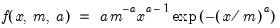
Syntax: @dweib(x, m, a)
x: number,

m: number,

a: number,

Return: number
Evaluates the probability density function,
for

and 0 elsewhere.
Examples
= @dweib(@log(2), 1, 1)
returns 0.5.
Cross-references
See also
@cweib,
@qweib, and
@rweib.
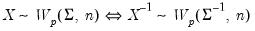
Wishart probability density.
Syntax: @dwish(X, S, n)
@dwishc(X, S, n)
@dwishi(X, S, n)
@dwishic(X, S, n)
X: sym,

S: sym, matrix,

n: number,

Return: number
Evaluate the Wishart distribution

density function for sym values of
X, and

.
The Wishart density is given by
where

and

are symmetric

matrices, and

.
There are four different forms of the density evaluation function, corresponding to different ways of specifying

. The forms are distinguished by different suffixes that are applied to the base “@dwish” command and how they change the interpretation of the
S matrix argument:
@dwish | “” | Supply  . |
@dwishc | “c” | Supply the Cholesky decomposition of  . This form is more efficient when performing multiple draws from the same distribution (compute the Cholesky once, but sample many times). |
@dwishi | “i” | Supply  . This form is more efficient than explicitly inverting  to supply  . |
@dwishic | “ic” | Supply the Cholesky decomposition of  . This form combines the efficiencies of the Cholesky and inverse forms. |
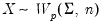
is generally thought of as the accumulated scatter matrix of
n random draws from

,
i.e.,

,
,
though the mathematical definition has been extended to cover real-valued n.
Note that if

is a Wishart random variable, then

follows an inverse Wishart distribution:
Examples
= @dwish(@identity(3), @identity(3), 5)
returns 0.00018....
Cross-references