Function Reference: R
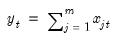
@range Vector of sequential integers.
@rapplyranks Reorder the columns of a matrix using a vector of ranks.
@rate Discount rate required for annuity to yield given present value.
@rbeta Beta distribution random draw.
@rbinom Binomial distribution random draw.
@rchisq Chi-square distribution random draw.
@regress Perform an OLS regression on the first column of a matrix versus the remaining columns.
@resample Randomly draw from the rows of the matrix.
@rexp Exponential distribution random draw.
@rextreme Extreme value (Type I-minimum) distribution random draw.
@rfdist F-distribution random draw.
@rfirst First non-missing value in rows of group object.
@rgamma Gamma distribution random draw.
@rged Generalized error distribution random draw.
@rifirst Indices of first non-missing value in rows of group object.
@right Right substring of string.
@rilast Indices of last non-missing value in rows of group object.
@rimax Indices of row maximums of group object.
@rimin Indices of row minimums of group object.
@rinstr Find substring position in string.
@riwish Inverse Wishart random draws.
@rlast Last non-missing values in rows of group object.
@rlognorm Log normal distribution random draw.
@rmax Row maximums of group object.
@rmean Row means of group object.
@rmin Row minimums of group object.
@rmse Root of the mean of square error (difference) between series.
@rmvnorm Multivariate normal random draws.
@rnas Number of missing observations in row of group object.
@rnegbin Negative binomial distribution random draw.
@rnorm Standard normal distribution random draw.
@robs Number of non-missing observations in row of group object.
@round Nearest integer, or value at given precision.
@rowranks Matrix where each row contains ranks of the column values.
@rowsort Matrix where each row contains sorted columns.
@rpareto Pareto distribution random draw.
@rprod Row products in group object.
@rstdev Row sample (d.f. corrected) standard deviations of group object.
@rstdevp Row population (non d.f. corrected) standard deviations of group object.
@rstdevs Row sample (d.f. corrected) standard deviations of group object.
@rsum Row sums of group object.
@rsumsq Row sums of squares of group object.
@rtdist Student’s

distribution random draw.
@rtrim Trim right whitespace of string.
@runif Uniform distribution random draw.
@runpath Location of the program currently being executed.
@rvalcount Number of matching values in rows of group object.
@rvar Row population (non d.f. corrected) variances of group object.
@rvarp Row population (non d.f. corrected) variances of group object.
@rvars Row sample (d.f. corrected) standard deviations of group object.
@rweib Weibull distribution random draw.
Vector of sequential integers.
Syntax: @range(n1, n2)
n1: integer
n2: integer
Return: vector
Returns a vector holding the sequential integers staring at n1 and ending at n2.
Examples
vector r1 = @range(1, 10)
create a vector containing sequential integers from 1 to 10.
vector r2 = @range(10, -3)
creates a vector containing integers starting at 10 and continuing to -3.
matrix m1a = m1.@sub(@range(3, m1.@rows), @range(2, m1.@cols))
extracts a submatrix from M1 starting at row 3 and column 2 and continuing to the end of the matrix.
matrix m1b = m1.@sub(@range(3, 7), @range(2, 4))
extracts a submatrix from M1 from row 3 to 7 and column 2 to 4.
Cross-references
Rank of the matrix.
Syntax: @rank(m[, n])
m: matrix, sym, vector, series
n: (optional) number
Return: integer
The rank of m is calculated by counting the number of singular values of the matrix which are smaller in absolute value than the tolerance, n.
If n is not provided, EViews uses the value given by the largest dimension of the matrix multiplied by the norm of the matrix multiplied by machine epsilon (the smallest representable number).
Examples
= @rank(m1)
returns the rank of the matrix M1. If M1 is a matrix of zeros, its rank is 0. If M1 is a matrix of a non-zero constant, its rank is 1.
Cross-references
To obtain a ranking of the elements in a matrix, see
@ranks as well as
@colranks and
@rowranks.
Ranking of values.
Determine the ranking associated with each value.
Syntax: @ranks(x[, y, z, s])
x: series, vector, matrix
y: (optional) string literal
z: (optional) string literal
s: (optional) sample string or object when x is a series
Return: series, vector, matrix object
The optional arguments control the behavior of the ranking procedure
The y option controls the direction of the ranking:
• “a” (ascending - default) or “d” (descending)
The z option controls tie-handling with rankings handled according to the setting:
• “i” (ignore), “f” (first), “l” (last), “a” (average - default), “r” randomize.
For series calculations, EViews will use the current or specified workfile sample.
Examples
vector y = @ranks(x, "a", "i")
returns the unique integer ascending ranking for the data in vector x, ignoring ties.
Cross-references
Reorder the columns of a matrix using a vector of ranks.
Syntax: @rapplyranks(m, v[, n])
m: matrix, vector
v: vector
n: (optional) integer
Return: matrix, vector
Apply (a row of) column ranks in the vector v to reorder the columns of a matrix m using the ranks.
• v should contain unique integers from 1 to the number of columns of m.
• If the optional argument n is specified, only the elements in row n will be reordered.
Examples
vector v1 = @ranks(m1.@row(3), "a", "i")
matrix m2 = @rapplyranks(m1, v1)
reorders the columns of the matrix M1 using the ranks in V1. Note that you may use the @ranks function to obtain the ranks of a vector but must obtain unique integer ranking for data with ties through use of the “i” or “r” option in @ranks.
matrix m3 = @rapplyranks(m1, v1, 3)
reorders only the elements in row 3 of M1.
Cross-references
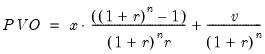
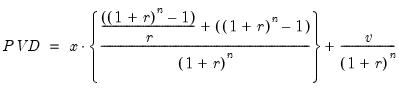
Discount rate required for annuity to yield given present value.
Syntax: @rate(n, x, pv[, v, bf])
n: integer
x: number
pv: number
v: (optional) number
bf: (optional) number
Return: number
Find the largest discount rate r producing at least the present value pv from an n-period annuity, with receipts x, and optional receipt of a final lump sum v.
If
n is not an integer, the integer floor

will be used.
A non-zero value for the optional bf indicates that the receipts are made at the beginning of periods (annuity due) instead of ends (ordinary annuity).
• The present value of by n-periods of ordinary annuity receipts and a final lump sum is:
• The present value of n-periods of annuity due receipts and a final lump sum is:
Then for a given PVO or PVD and annuity type, the function returns the largest discount rate r where the present values still exceed the required value.
Examples
= @rate(15, 100, 1000)
returns the value 0.055565, indicating that a 15-year annuity that pays $100 per period has a present value of $1000 if the discount rate is set to 0.055565.
Cross-references
See also
@fv,
@nper,
@pmt, and
@pv.
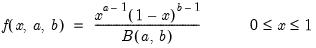
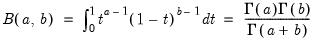
Beta distribution random draw.
Syntax: @rbeta(x, a, b)
x: number
a: number,

b: number,

Return: number
Draw a random value from the beta distribution with density function,
and 0 elsewhere, where

is the beta function
Examples
= @rbeta(1, 2)
returns a random draw from the Beta(1, 2) distribution.
Cross-references
See also
@cbeta,
@dbeta, and
@qbeta.
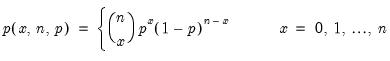
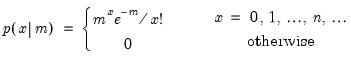
Binomial distribution random draw.
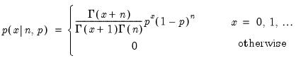
Syntax: @rbinom(n, p)
n: integer,

p: number,

Return: integer
Draw a random integer value from the binomial distribution with probability function,
and 0 elsewhere.
Examples
= @rbinom(5, 0.5)
returns a random draw from the Binom(5, 0.5) distribution.
Cross-references
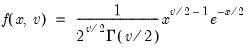
Chi-square distribution random draw.
Syntax: @rchisq(v)
v: number,

Return: number
Draw a random value from the chi-square distribution with density function,
Examples
= @rchisq(10)
returns a random draw from the chi-square distribution with 10 degrees of freedom.
Cross-references
Recode value by condition.
Returns

if condition

is non-zero (true); otherwise returns

.
Syntax: @recode(s, x, y)
s: number
x: number or string
y: number or string
Return: number or string
Returns

if

is non-zero (true); otherwise returns

.
Typically

is specified using an expression with a boolean operator or function returning (0, 1) values (
e.g., “z > 3”or “z > w”), but any argument providing (0, non-zero) values is sufficient.
Examples
= @recode(x<0, 1, 0)
returns 1 if x is negative, 0 otherwise.
Cross-references
Perform an OLS regression on the first column of a matrix versus the remaining columns.
Syntax: @regress(m[, v])
m: matrix
v: (optional) vector
Return: matrix
Returns the results of an OLS regression on the first column of matrix m versus the remaining columns of m.
The returned matrix contains four columns of information: (1) regression coefficient values, (2) standard errors, (3) t-test statistics, and (4) associated p-values.
If an optional vector v is supplied, the regression residuals are stored in v.
Examples
matrix results = @regress(yxmat)
estimates a regression on the data in the columns of the matrix YXMAT and saves the coefficient, standard error, t-statistic and p-value results in columns of RESULTS
Next for comparison purposes we run a regression on random data using the equation object, collect results in a matrix, and make a series containing the residuals.
First, create a workfile with random data, create a group with the dependent variable and regressors, and set the workfile sample.
workfile q 2000 2022
series y = nrnd
series x1 = nrnd
series x2 = nrnd
group yx y 1 x1 x2
smpl 2002 2022
equation eq1.ls y c x1 x2
matrix eq_results = @hcat(eq1.@coefs, eq1.@stderrs, eq1.@tstats, eq1.@pvals)
eq1.makeresids eq_resids
The function offers a quick way of obtaining equivalent results,
vector fn_resids
matrix fn_results = @regress(@convert(yx), fn_resids)
Cross-references
Replace substring in string.
Syntax: @replace(str1, str2, str3[, n])
str1: string, alpha, svector
str2: string, alpha, svector
str3: string, alpha, svector
n: (optional) integer, series, vector
Return: string, alpha, svector
Returns the base string str1, with the str3 substituted for the target string str2. By default, all occurrences of str2 will be replaced, but you may provide an optional integer n to specify the maximum number of occurrences to be replaced.
Examples
@replace("Do you think that you can do it?", "you", "I")
returns the string “Do I think that I can do it?”, while
@replace("Do you think that you can do it?", "you", "I", 1)
only replaces the first instance of “you” with “I” so that it returns “Do I think that you can do it?”.
If ALPHA1 is an alpha series,
alpha a1 = @replace(alpha1, "abc", "def")
replaces all instances of “abc” with “def” in ALPHA1 for all observations in the workfile sample.
If AVEC1 and AVEC2 are string vectors,
svector s1 = @replace(avec1, avec2, "abc")
replaces all instances of the strings in AVEC2 with “abc” for each element of AVEC1.
Cross-references
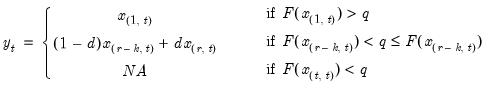
Randomly draw from the rows of the data object.
Syntax: @resample(m[, n1, n2, v])
m: data object
n1: (optional) integer
n2: (optional) positive integer
v: (optional) vector
Output: data object
Returns a data object whose rows are randomly drawn with replacement from rows of the input matrix or vector.
By default, the output matrix will be the same size as the source m.
• 
represents the number of “extra” rows to be drawn from the matrix. If the input matrix has
r rows and
c columns, the output matrix will have

rows and

columns. By default,

.
• 
represents the block size for the resample procedure. If you specify

, then blocks of consecutive rows of length

will be drawn with replacement from the first

rows of the input matrix.
• You may provide a name for the vector

to be used for weighted resampling. The weighting vector must have length

and all elements must be non-missing and non-negative. If you provide a weighting vector, each row of the input matrix will be drawn with probability proportional to the weights in the corresponding row of the weighting vector. (The weights need not sum to 1. EViews will automatically normalize the weights).
To draw without replacement from rows of a matrix, use
@permute.
Examples
matrix xb = @resample(x)
yields the matrix XB whose rows were randomly sampled with replacement from the matrix X.
Cross-references
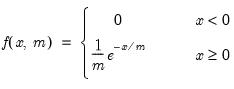
Exponential distribution random draw.
Syntax: @rexp(m)
m: number,

Return: number
Draw a random value from the exponential distribution with probability density function,
Examples
= @rexp(1)
returns a random draw from the exponential distribution with mean 1.
Cross-references
See also
@cexp,
@dexp, and
@qexp.
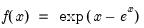
Extreme value (Type I-minimum) distribution random draw.
Syntax: @extreme
Return: number
Draw a random value from the extreme value distribution with probability density function,
Examples
= @rextreme
returns a random draw from the extreme value distribution.
Cross-references
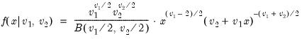
F-distribution random draw.
Syntax:
@rfdist(
 ,
,  )
) 
: number,


: number,

Return: number
Draw a random value from the F-distribution with density function,
for

and 0 otherwise, where

is the beta function,
Examples
= @rfdist(2, 2)
returns a random draw from the F-distribution with numerator and denominator degrees of freedom 2.
Cross-references
First non-missing value in rows of group.
Value of the first non-missing value in each row of the group.
Syntax: @rfirst(x)
x: group
Return: series
For each observation

corresponding to a row

in the group of

series, find the first non-missing value in the row.
Examples
show @rfirst(g
returns a linked series of the first non-missing observations in the rows of group g.
Cross-references
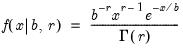
Gamma distribution random draw.
Syntax: @rgamma(b, r)
b: number,

r: number,

Return: number
Draw a random value from the gamma distribution with the probability density function,
for

, and 0 elsewhere.
Examples
= @rgamma(4, 1)
returns a random draw from the Gamma(4, 1) distribution.
Cross-references
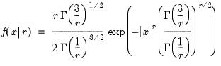
Generalized error distribution random draw.
Syntax: @rged(r)
r: number,

Return: number
Draw a random value from the generalized error distribution with density function,
Examples
= @rged(2)
returns a random draw from the Generalized error distribution.
Cross-references
See also
@cged,
@dged, and
@qged.
Indices of first non-missing value in rows of group.
Column indices of first non-missing value in each row of the group.
Syntax: @rifirst(x)
x: group
Return: series
For each observation

corresponding to a row

in the group of

series, identify the column containing the first non-missing value in the row.
Examples
show @rifirst(g
returns a linked series of the indices corresponding to the first non-missing observations in the rows of group g.
Cross-references
Right substring of string.
Syntax: @right(str, n)
str: string, alpha, svector
n: integer, series, vector
Return: string, alpha, svector
Returns a string containing n characters from the right end of str. If the source is shorter than n, the entire string is returned.
Examples
The commands
string orig = "I doubt it"
string sc1 = @right("I doubt it", 8)
string sc2 = @left(orig, 8)
return the string objects SC1 and SC2 containing the string “doubt it”.
If ALPHA1 is an alpha series,
alpha strleft = @right(alpha1, 7)
returns the right-most 7 characters from the string values of ALPHA1 for each observation in the workfile sample.
If SVEC1 is an string vector,
svector strleft = @right(svec1, 12)
returns an svector containing 12 characters from the right end of each element of SVEC1.
Cross-references
Indices of last non-missing value in rows of group.
Column indices of last non-missing value in each row of the group.
Syntax: @rilast(x)
x: group
Return: series
For each observation

corresponding to a row

in the group of

series, identify the column containing the last non-missing value in the row.
Examples
show @rilast(g
returns a linked series of the indices corresponding to the last non-missing observations in the rows of group g.
Cross-references
Indices of row maximums of group.
Column indices of maximum values across series in each row of the group.
Syntax: @rimax(x)
x: group
Return: series
For each observation

corresponding to a row

in the group of

series, identify the column containing the maximum value across the data for the row.
Examples
show @rimax(g
returns a linked series of the indices corresponding to the maximums in the rows of group g.
Cross-references
See also
@rmax,
@rmin, and
@rimin.
Indices of row minimums of group.
Column indices of minimum values across series in each row of the group.
Syntax: @rimin(x)
x: group
Return: series
For each observation

corresponding to a row

in the group of

series, identify the column containing the minimum value across the data for the row.
Examples
show @rimin(g
returns a linked series of the indices corresponding to the minimums in the rows of group g.
Cross-references
See also
@rmax,
@rmin, and
@rimax.
Find substring position in string, search in reverse.
Syntax: @rinstr(str1, str2[, n])
str1: string, alpha
str2: string, alpha
n: (optional) integer, series
Return: integer, series
Starting at the end of the string and searching in reverse, finds the starting position of the target string str2 in the string str1. By default, the function returns the location of the last (first from the end) instance of str2 in str1, but you may provide the optional integer n to change the occurrence.
If the target string is not found, @rinstr will return a 0.
Examples
string sval = "1.2341534"
@rinstr("1.2341534", "34")
@instr(sval, "34")
return the value 4, since the substring “34” appears a second time (from the end of the string) beginning in the fourth character of the base string.
If ALPHA1 is an alpha series,
series strfind = @rinstr(alpha1, "34")
fills the series with the last location (first from the end of the string) of the string “34” in each string in ALPHA1, for each observation in the workfile sample.
Cross-references
See also
@instr for finding substrings starting from the beginning of the string, and
@mid for extracting substrings.
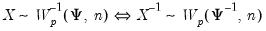
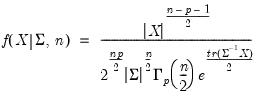
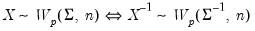
Inverse Wishart random draws.
Syntax: @riwish(S, n)
@riwishc(S, n)
@riwishi(S, n)
@riwishic(S, n)
@riwish(X, S, n)
@riwishc(X, S, n)
@riwishi(X, S, n)
@riwishic(X, S, n)
X: (optional) sym,

S: sym, matrix,

n: number,

Return: sym
Draw a random symmetric inverse Wishart matrix using the

density function.
The inverse Wishart density is given by
 | (18.8) |
where

and

are symmetric

matrices, and

.
There are four different forms of the function, corresponding to different ways of specifying

. The forms are distinguished by different suffixes that are applied to the base “@
rwish” command and how they change the interpretation of the
S matrix argument:
@riwish | “” | Supply  . |
@riwishc | “c” | Supply the Cholesky decomposition of  . This form is more efficient when performing multiple draws from the same distribution (compute the Cholesky once, but sample many times). |
@riwishi | “i” | Supply  . This form is more efficient than explicitly inverting  to supply  . |
@riwishic | “ic” | Supply the Cholesky decomposition of  . This form combines the efficiencies of the Cholesky and inverse forms. |
Note that if

is an inverse Wishart random variable, then

is follows a Wishart distribution:
Examples
= @riwish(@identity(3), 5)
returns a random draw from the

distribution.
Cross-references
Laplace distribution random draw.
Syntax: @rlaplace
Return: number
Draw a random value from the Laplace distribution with probability density function,
Examples
= @rlaplace
returns a random draw from the Laplace distribution.
Cross-references
Last non-missing values in rows of group.
Value of the last non-missing value in each row of the group.
Syntax: @rlast(x)
x: group
Return: series
For each observation

corresponding to a row

in the group of

series, find the last non-missing value in the row.
Examples
show @rlast(g
returns a linked series of the last non-missing observations in the rows of group g.
Cross-references
Logistic distribution random draw.
Syntax: @rlogistic
Return: number
Draw a random value from the logistic distribution with probability density function,
Examples
= @rlogistic
returns a random draw from the logistic distribution.
Cross-references
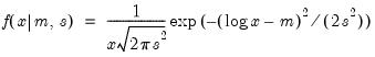
Log normal distribution random draw.
Syntax: @rlognorm(m, s)
m: number,

s: number,

Return: number
Draw a random value from the log normal error distribution with density function,
for

and 0 otherwise.
Examples
= @rlognorm(0, 2)
returns a random draw from the log-normal(0, 2) distribution.
Cross-references
Row maximums of group.
Maximum values across series in each row of the group.
Syntax: @rmax(x)
x: group
Return: series
For each observation

corresponding to a row

in the group of

series, find the maximum value across the data for the row.
Examples
show @rmax(g
returns a linked series of the maximums in the rows of group g.
Cross-references
See also
@rmin,
@rimax, and
@rimin.
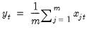
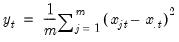
Row means of group.
Mean value across series in each row of the group.
Syntax: @rmeans(x)
x: group
Return: series
For each observation

corresponding to a row

in the group of

series, compute the mean of the values,
Examples
show @rmean(g
returns a linked series of the means in the rows of group g.
Cross-references
See also
@rmedian and
@rvar.
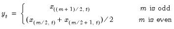
Row median of group.
Medians for each row of the group.
Syntax: @rmedian(x)
x: group
Return: series
For each observation

corresponding to a row in the group of

series, compute the median of the

values

for the observation.
When

is odd, the median is the middle ordered-observation and when

is even, the median is the average of the two middle ordered-observations. The median may be written as
where the order statistics
represent the data for observation

ordered from low to high.
Examples
show @rmedian(g
returns a linked series of the medians in the rows of group g.
Cross-references
Row minimums of group.
Minimum values across series in each row of the group.
Syntax: @rmin(x)
x: group
Return: series
For each observation

corresponding to a row

in the group of

series, find the minimum value across the data for the row.
Examples
show @rmin(g
returns a linked series of the minimums in the rows of group g.
Cross-references
See also
@rmax,
@rimax, and
@rimin.
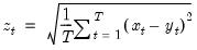
Root of the mean of square error (difference) between series.
Computes the square root of the mean of the squared difference between x and y.
Syntax: @rmse(x, y, [s])
x: series
y: series
s: (optional) sample string or object
Return: number
Examples
Let yf denote in-sample forecasts for the series y. Then
= @rmse(yf, y)
returns the RMSE between the series y and its forecast.
Cross-references
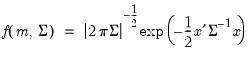
Multivariate normal random draws.
Syntax: @rmvnorm(S[, n])
@rmvnormc(S[, n])
@rmvnormi(S[, n])
@rmvnormic(S[, n])
m: (optional) vector
S: sym, matrix
n: (optional) integer,

Return: vector, matrix
Draw random multivariate normals using the

density function.
The multivariate normal density is given by
There are four different forms of the function, corresponding to different ways of specifying

. The forms are distinguished by different suffixes that are applied to the base “@rmvnorm” command and how they change the interpretation of the
S matrix argument:
@rmvnorm | “” | Supply  . |
@rmvnormc | “c” | Supply the Cholesky decomposition of  . This form is more efficient when performing multiple draws from the same distribution (compute the Cholesky once, but sample many times). |
@rmvnormi | “i” | Supply  . This form is more efficient than explicitly inverting  to supply  . |
@rmvnormic | “ic” | Supply the Cholesky decomposition of  . This form combines the efficiencies of the Cholesky and inverse forms. |
If the optional argument n is omitted, the function returns a vector containing a single draw from the distribution. If n is provided, n is the number of rows of the returned matrix, with each row representing a draw from the distribution.
Examples
= @dmvnorm(@identity(3))
returns a random draw from a trivariate normal distribution.
Cross-references
Number of missing observations in row of group.
Number of missing observations in each row of the group.
Syntax: @rnas(x)
x: group
Return: series
For each observation

corresponding to a row

in the group of

series, count the number of missing (NA) observations.
Examples
show @rnas(g
returns a linked series of the NA counts in the rows of group g.
Cross-references
See also
@robs and
@rvalcount.
Negative binomial distribution random draw.
Syntax: @rnegbin(n, p)
n: number,

p: number,

Return: integer
Draw a random integer value from the negative binomial distribution with probability function,
Examples
= @rnegbin(10, 0.5)
returns a random draw from the negative binomial(10, 0.5) distribution.
Cross-references
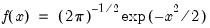
Standard normal distribution random draw.
Syntax: @rnorm
Return: number
Draw a random value from the standard normal distribution with probability density function,
Examples
= @rnorm
returns a random draw from the standard normal distribution.
Cross-references
Row numbers of non-missing observations in group.
Number of non-missing observations in each row of the group.
Syntax: @robs(x)
x: group
Return: series
For each observation

corresponding to a row

in the group of

series, count the number of non-missing observations.
Examples
show @robs(g
returns a linked series of the non-NA counts in the rows of group g.
Cross-references
See also
@rnas and
@rvalcount.
Nearest integer, or value at given precision.
Return nearest integer or nearest decimal number at the given precision.
Syntax: @round(x[, n])
x: number
n: (optional) integer
Return: number
The decimal offset n may be interpreted as the precision to use when rounding the number.
• @round(x) returns the nearest integer to x. Numbers exactly midway between integers (e.g., 1.5 or 37.5) are rounded to next higher integer.
• @round(x, n) rounds to the nearest decimal number to x at the given precision:

.
If
n is not an integer, the integer floor

will be used.
Examples
= @round(-97.5)
returns -98.
= @round(@pi, 3)
returns 3.142.
Cross-references
See also
@ceil and
@floor.
Extract rowvector from matrix object.
Syntax: @rowextract(m, n)
m: matrix, sym
n: integer
Return: vector
Extract a vector from row n of the matrix object m, where m is a matrix object.
Note that we recommend that extraction be performed using the newer “.row” object data member functions. See
“Matrix Data Members” and
“Sym Data Members” and the examples below.
Examples
matrix m1 = @mnrnd(20, 5)
vector v1 = @rowextract(m1,3)
extracts row 3 from the matrix M1.
sym s1 = @unvech(@mnrnd(15))
vector v2 = @rowextract(s1, 5)
Alternately, using the data member functions, we have
vector v1a = m1.@row(3)
vector v1b = s1.@row(5)
Cross-references
Matrix where each row contains ranks of the column values.
Syntax: @rowranks(m[, o, t])
m: matrix, vector
o: (optional) string
t: (optional) string
Return: matrix, vector
Returns a matrix where each row contains the rankings of the values of the corresponding row of m.
The o option controls the direction of the ranking:
• “a” (ascending - default) or “d” (descending).
The t option controls tie-handling:
• Ties are broken according to the setting of t: “i” (ignore), “f” (first), “l” (last), “a” (average - default), “r” randomize.
If you wish to specify tie-handling options, you must also specify the order option (e.g., @rowranks(x, "a", "i")).
Examples
= @rowranks(m1, "d")
returns a matrix whose i-th row ranks the elements in the i-th row of M1 so that the largest element in said row has a rank of 1.
Cross-references
See also
@ranks and
@colranks.
Number of rows.
Syntax: @rows(m)
m: matrix, vector, sym, series, group
Return: integer
For series and groups @rows returns the number of observations in the workfile range.
Examples
matrix m1 = @mnrnd(10, 3)
scalar sc2 = @rows(m1)
assigns the value 10 to the scalar object SC2.
series q = nrnd
series r = nrnd
series s = nrnd
series t = nrnd
group mygrp q r s t
vector g = @fill(@rows(q), @columns(mygrp))
creates a two-element vector G containing the number of rows of Q and the number of series in MYGRP.
Cross-references
Matrix where each row contains sorted columns.
Syntax: @rowsort(m[, o])
m: matrix, vector
o: (optional) string
Return: matrix, vector
Returns a matrix where each row contains the sorted values of the corresponding row of m.
The option o controls the direction of the ranking: “a” (ascending - default) or “d” (descending).
Examples
Let M1 be a matrix. Then
= @rowsort(m1, "d")
returns a matrix whose i-th row is the sorted (from largest on the left to smallest on the right) version of the i-th row in M1.
Cross-references
See also
@sort and
@colsort.
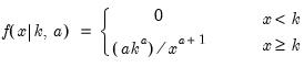
Pareto distribution random draw.
Syntax: @rpareto(k, a)
k: number,

a: number,

Return: number
Draw a random value from the Pareto distribution with probability density function,
Example
= @rpareto(1, 2)
returns a random draw from the Pareto(1, 2) distribution.
Cross-references
Poisson distribution random draw.
Syntax: @rpoisson(m)
m: number,

Return: integer
Draw a random integer value from the Poisson distribution with probability function,
Examples
= @rpoisson(10)
returns a random draw from the Poisson(10) distribution.
Cross-references
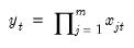
Row products in group.
Product across series in each row of the group.
Syntax: @rsum(x)
x: group
Return: series
For each observation

corresponding to a row
in the group of

series, compute the product of the values,
Note that this function is prone to numeric overflow.
Examples
show @rprod(g
returns a linked series of the products of observations in the rows of group g.
Cross-references
Row quantiles in group.
Quantiles for each row of the group.
Syntax: @rquantile(x, q)
x group
q number, series
Return: series
For each observation

corresponding to a row in the group of

series, compute the
q-quantile of the

values

for the observation using the Rankit-Cleveland quantile definition, for

.
To compute the

-quantile, first find

, the smallest rank such that,
where the order statistics

represent data for the

series ordered from low to high, and

is the Rankit-Cleveland definition of the empirical distribution function:
. For purposes of computing

, tied ranks are assumed to take the last tied value.
Then the quantile is computed as
where the interpolating constant is
for

the smallest integer where
. In the leading case where there are no tied

values,

.
Examples
show @rquantile(g, 0.25
returns a linked series of the 25th percentiles in the rows of group g.
Cross-references
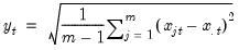
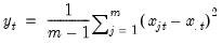
Row sample (d.f. corrected) standard deviations.
Square roots of the Pearson product moment sample variances for each row of the group, with d.f. correction.
Syntax: @rstdev(x)
x: group
Return: series
For each observation

corresponding to a row in the group of

series, compute the sample standard deviation,
where

is the mean of the

values

for the observation.
Examples
show @rstdev(g
returns a linked series of sample standard deviations in the rows of group g.
Cross-references
Row population (non d.f. corrected) standard deviations.
Square roots of (population) Pearson product moment population variances for each row of the group, with no d.f. correction.
Syntax: @rstdevp(x)
x: group
Return: series
For each observation

corresponding to a row in the group of

series, compute the population standard deviation,
where

is the mean of the

values

for the observation.
Examples
show @rstdevp(g
returns a linked series of population standard deviations in the rows of group g.
Cross-references
See also
@rstdev and
@rstdevs.
Row sample (d.f. corrected) standard deviations.
Square roots of Pearson product moment sample variances for each row of the group, with d.f. correction.
Syntax: @rstdevs(x)
x: group
Return: series
For each observation

corresponding to a row in the group of

series, compute the sample standard deviation,
where

is the mean of the

values

for the observation.
Equivalent to @rstdev.
Examples
show @rstdevs(g
returns a linked series of sample standard deviations in the rows of group g.
Cross-references
See also
@rstdev and
@rstdevp.
Row sums.
Sum across series in each row of the group.
Syntax: @rsum(x)
x: group
Return: series
For each observation

corresponding to a row

in the group of

series, compute the sum of the values,
Examples
show @rsum(g
returns a linked series of the sums of observations in the rows of group g.
Cross-references
See also
@rprod and
@rsumsq.
Row sums of squares.
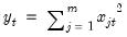
Sums of squared values for each row of the group
Syntax: @rsumsq(x)
x: group
Return: series
For each observation

corresponding to a row

in the group of

series, compute the sum of squared values,
Examples
show @rsumsq(g
returns a linked series of the sums of squares in the rows of group g.
Cross-references
Reverse sweep operator.
There are two syntaxes for @rsweep, one for the symmetric, and the other for then non-symmetric operator.
Syntax: @rsweep(s[, n])
s: sym
k: integer
k2: (optional) integer
Return: matrix
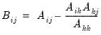
Returns the result of applying the symmetric sweep operator to symmetric matrix S at diagonal element k. If k2 is specified, sweeps on all diagonal elements between k and k2, inclusive.
This is merely an alias for @sweep(s, k[, k2]), since the symmetric sweep operator is its own reverse/inverse.
Syntax: @rsweep(m, r, c)
m: matrix, sym
r: integer
c: integer
Return: matrix
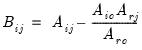
Returns the result of applying the reverse non-symmetric sweep operator to general matrix M at element (r, c).
Let
be an application of the symmetric sweep operator. Then,
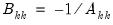
,
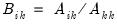
where

,
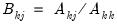
where

, and
where

and

.
Let
be an application of the non-symmetric sweep operator. Then,
,
where

,

where

, and
where

and

.
Examples
Consider a swept matrix replicating the results of an OLS regression (see @sweep function).
group g y x1 x2 x3
sym usscp = @inner(g)
sym s = @sweep(usscp, 2, 4)
Just as each application of the sweep operator effectively switched the role of a variable from dependent to regressor, each application of the reverse sweep operator switches the role of a variable from regressor back to dependent.
For example, we can remove X1 as a regressor for Y by applying @rsweep to the corresponding diagonal element.
s = @rsweep(s, 2, 2)
We can also verify these results against a standard equation object:
vector beta = @subextract(S, 3, 1, 4, 1) ' Regressor coefficients
scalar ssr = s(1,1) ' Sum of squared residuals
sym invXtX = -@subextract(s, 3, 3)
vector se = @sqrt(ssr * @getmaindiagonal(invXtX) / (@obssmpl - 2)) ' Coefficient standard errors
equation eq.ls(noconst) y x2 x3
Cross-references
Goodnight, James H. (1979). “A Tutorial on the SWEEP Operator,” The American Statistician, 33, 149–158.
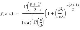
Student’s

distribution random draw.
Syntax: @rtdist(v)
v: number,

Return: number
Draw a random value from the Student’s

distribution with probability density function,
Examples
= @rtdist(1)
returns a random draw from the Cauchy distribution.
Cross-references
Trim right whitespace of string.
Syntax: @rtrim(str)
str: string, alpha, svector
Return: string, alpha, svector
Returns the string str with spaces trimmed from the right.
Examples
@rtrim(" I doubt that I did it. ")
returns the string “ I doubt that I did it.”. Note that the spaces on the left remain.
If ALPHA1 is an alpha series,
alpha alphaltrim = @rtrim(alpha1)
returns the right-trimmed strings in ALPHA1 for each observation in the workfile sample.
If SVEC1 is an string vector,
svector sveclen = @ltrim(svec1)
returns a string vector containing the right-trimmed elements of SVEC1.
Cross-references
See also
@ltrim and
@trim.
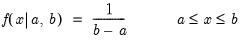
Uniform distribution random draw.
Syntax: @runif(a, b)
a: number
b: number,

Return: number
Draw a random value from the uniform distribution with probability density function,
and 0 otherwise.
Examples
= @runif(1, 6)
returns a random draw from the continuous uniform(1, 6) distribution.
Cross-references
See also
@cunif,
@dunif, and
@qunif.
Syntax: @runpath
Return: string
Returns a string containing the location of the program currently being executed. If @runpath is being executed as a child program from a parent as part of an include or exec statement, the string will return the location of the parent program.
Examples
If the program d:\myprogs\program1.prg has the line:
string y = @runpath
then y will contain “D:\MYPROGS\PROGRAM1.PRG”, if program1 is run by itself, and will return the location of the parent program otherwise.
Cross-references
Number of matching values in rows.
Syntax: @rvalcount(x, v)
x: group
v: number, series
Return: series
The number of observations with a value equal to v in each row of the group.
Examples
show @rvalcount(g, 1)
returns a linked series of counts of the number 1 in the rows of group g.
Cross-references
See also
@rnas and
@robs.
Row population (non d.f. corrected) variances.
Pearson product moment population variances for each row of the group, with d.f. correction.
Syntax: @rvars(x)
x: group
Return: series
For each observation

corresponding to a row in the group of

series, compute the population variance,
where

is the mean of the

values

for the observation.
Examples
show @rvar(g
returns a linked series of population variances in the rows of group g.
Cross-references
See also
@rvarp and
@rvars.
Row population (non d.f. corrected) variances.
Pearson product moment population variances for each row of the group, with d.f. correction.
Syntax: @rvars(x)
x: group
Return: series
For each observation

corresponding to a row in the group of

series, compute the population variance,
where

is the mean of the

values

for the observation.
Examples
show @rvarp(g
returns a linked series of population variances in the rows of group g.
Cross-references
See also
@rvar and
@rvars.
Row sample (d.f. corrected) standard deviations.
Pearson product moment population variances for each row of the group, with d.f. correction.
Syntax: @rvars(x)
x: group
Return: series
For each observation

corresponding to a row in the group of

series, compute the sample variance,
where

is the mean of the

values

for the observation.
Examples
show @rvars(g
returns a linked series of sample variances in the rows of group g.
Cross-references
See also
@rvar and
@rvarp.
Weibull distribution random draw.
Syntax: @rtdist(m, a)
m: number,

a: number,

Return: number
Draw a random value from the Weibull distribution with probability density function,
for

and 0 elsewhere.
Examples
= @rweib(1, 1)
returns a random draw from the Weibull(1, 1) distribution.
Cross-references
See also
@cweib,
@dweib, and
@qweib.
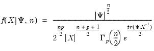
Wishart random draw.
Syntax: @rwish(S, n)
@rwishc(S, n)
@rwishi(S, n)
@rwishic(S, n)
X: (optional) sym,

S: sym, matrix,

n: number,

Return: sym
Draw a random symmetric Wishart matrix using the

density function.
The Wishart density is given by
where

and

are symmetric

matrices, and

.
There are four different forms of the function, corresponding to different ways of specifying

. The forms are distinguished by different suffixes that are applied to the base “@
rwish” command and how they change the interpretation of the
S matrix argument:
@rwish | “” | Supply  . |
@rwishc | “c” | Supply the Cholesky decomposition of  . This form is more efficient when performing multiple draws from the same distribution (compute the Cholesky once, but sample many times). |
@rwishi | “i” | Supply  . This form is more efficient than explicitly inverting  to supply  . |
@rwishic | “ic” | Supply the Cholesky decomposition of  . This form combines the efficiencies of the Cholesky and inverse forms. |
is generally thought of as the accumulated scatter matrix of
n random draws from

,
i.e.,

,
,
though the mathematical definition has been extended to cover real-valued n.
Note that if

is a Wishart random variable, then

follows an inverse Wishart distribution:
Examples
= @rwish(@identity(3), 5)
returns a random draw from the

distribution.
Cross-references