There are several ways to create a matrix object. You can enter the matrix keyword (with an optional row and column dimension) followed by a name:

Alternatively, you can combine a declaration with an assignment statement, in which case the new matrix will be sized accordingly.

Lastly, a number of object procedures create matrices.

Graph creation views are discussed in detail in “Graph Creation Command Summary”.

The following assignment statements create and initialize matrix objects,

as does the equation procedure:

You can declare and initialize a matrix in one command:

Graphs and covariances may be generated for the columns of the matrix,

and statistics computed for the rows of a matrix:

You can use explicit indices to refer to matrix elements:

clears the custom column labels from the matrix MAT1.

See also Matrix::clearrowlabels.

Removes the matrix’s history attribute, as shown in the label view of the matrix.

The first line removes the history from the matrix M1, and the second line displays the label view of M1, including the now blank history field.

See “Labeling Objects” for a discussion of labels and display names.

See also Matrix::label.

Removes the matrix’s remarks attribute, as shown in the label view of the matrix.

The first line removes the remarks from the matrix M1, and the second line displays the label view of M1, including the now blank remarks field.

See “Labeling Objects” for a discussion of labels and display names.

See also Matrix::label.

clears the custom row labels from the matrix MAT1.

See also Matrix::clearcollabels.

Creates either a named or unnamed copy of the matrix.

creates an unnamed copy of the matrix M1.

creates M2, a copy of the matrix M1.

See also copy.

You may compute measures related to Pearson product-moment (ordinary) covariances and correlations, Spearman rank covariances, or Kendall’s tau along with test statistics for evaluating whether the correlations are equal to zero.

You should specify keywords indicating the statistics you wish to display from the list below, optionally followed by the keyword @partial and the name of a conditioning matrix. The columns should contain the conditioning variables, and the number of rows should match the original matrix.

You may specify keywords from one of the four sets (Pearson correlation, Spearman correlation, Kendall’s tau, Uncentered Pearson) corresponding the computational method you wish to employ. (You may not select keywords from more than one set.)

If you do not specify keywords, EViews will assume “corr” and compute the Pearson correlation matrix. Note that Matrix::cor is equivalent to the Matrix::cov command with a different default setting.

Note that cases, obs, and wgts are available for each of the methods.

displays a table containing the Pearson correlation, t-statistic for testing for zero correlation, and associated p-value, for the columns in MAT1.

computes the Kendall’s tau-b, score statistic, and p-value for the score statistic, using samples with pairwise missing value exclusion.

computes the Pearson covariance for the columns in MAT1 and saves the results in the symmetric matrix object AACO.

See also Matrix::cov. For simple forms of the calculation, see @cor, and @cov.

You may compute measures related to Pearson product-moment (ordinary) covariances and correlations, Spearman rank covariances, or Kendall’s tau along with test statistics for evaluating whether the correlations are equal to zero.

You should specify keywords indicating the statistics you wish to display from the list below, optionally followed by the keyword @partial and the name of a conditioning matrix. The columns should contain the conditioning variables, and the number of rows should match the original matrix.

You may specify keywords from one of the four sets (Pearson correlation, Spearman correlation, Kendall’s tau, Uncentered Pearson) corresponding the computational method you wish to employ. (You may not select keywords from more than one set.)

If you do not specify keywords, EViews will assume “cov” and compute the Pearson covariance matrix. Note that Matrix::cov is equivalent to the Matrix::cor command with a different default setting.

Note that cases, obs, and wgts are available for each of the methods.

displays a table containing the Pearson covariance, t-statistic for testing for zero correlation, and associated p-value, for the columns in MAT1.

computes the Kendall’s tau-b, score statistic, and p-value for the score statistic, using samples with pairwise missing value exclusion.

computes the Pearson covariance for the columns in MAT1 and saves the results in the symmetric matrix object AACO.

See also Matrix::cor. For simple forms of the calculation, see @cor, and @cov.

Display the contents of a table, graph, or spool in the window of the matrix object.

Display the contents of the table TAB1 in the window of the object MATRIX1.

Most often used in constructing an EViews Add-in. See “Custom Object Output”.

Attaches a display name to a matrix object which may be used to label output in place of the standard matrix object name.

Display names are case-sensitive, and may contain a variety of characters, such as spaces, that are not allowed in matrix object names.

The first line attaches a display name “Hours Worked” to the matrix object M1, and the second line displays the label view of M1, including its display name.

See “Labeling Objects” for a discussion of labels and display names.

See also Matrix::label.

Saves the data used to display the kernel regression, nearest neighbor regression, or empirical quantile-quantile plot to the workfile.

saves the distribution plot data specified by dist_type where dist_type must be one of the following keywords:

The matrix_name_pattern is used to define a naming pattern for the output matrices; if the pattern is “NAME”, the resulting matrices will be named “NAME01”, “NAME02”, … and so on, using the next available name.

For the first two types (“kernfit” and “nnfit”), dist_options are any of the distribution type-specific options described in “Kernfit Options” and “Nnfit Options”, respectively. The empirical quantile-quantile plot type (“empqq”) takes the options described in qqplot under “Empirical Options”.

Note that the graph display specific options such as “fill,” “nofill,” “leg,” and “noline” are not relevant for this procedure.

In addition, you may use the “mult” option to specify multiple series handling

and the “prompt” option to force the dialog display

If MAT1 is a matrix with four columns,

then creates three matrices, M01, M02 and M03, where the M01 contains the kernel fit (with an Epanechnikov kernel and 100 grid points) of the second column of MAT1 on the first column, M02 contains the fit of the first column on the third column, and M03 contains the kernel fit of column 1 on column 4.

creates two matrices, N1 and N2, where N1 contains the nearest neighbor fit of column 1 on column 2 computed using a bandwidth of 0.3 and polynomial degree of 1, 100 evaluation points and symmetric neighbors, and N2 contains the data for the nearest neighbor fit of column 3 on column 4.

If we extract a new matrix MAT2 containing first three columns of MAT1, the commands

creates 3 matrices; MAT01, MAT02, and MAT03, where MAT01 contains the empirical quantile-quantile for columns 1 and 2, computed using the rankit quantile method, MAT02 contains the qq-plot data for columns 1 and 3, and MAT03 contains the qq-plot data for columns 2 and 3.

For a description of distribution graphs and quantile-quantile graphs, see “Auxiliary Graph Types”.

See also qqplot and “Auxiliary Spec”.

Follow the keyword with a name for the file. file_name may include the file type extension, or the file type may be specified using the “t=” option.

If an explicit path is not specified, the file will be stored in the default directory, as set in the File Locations global options.

The base syntax for writing Excel 2007 files is:

where the table_description may contain:

If the worksheet name contains spaces, it should be placed in single quotes. If the worksheet name is omitted, the cell range is assumed to refer to the currently active sheet. If only a top left cell is provided, a bottom right cell will be chosen automatically to cover the range of non-empty cells adjacent to the specified top left cell. If only a sheet name is provided, the first set of non-empty cells in the top left corner of the chosen worksheet will be selected automatically. As an alternative to specifying an explicit range, a name which has been defined inside the Excel workbook to refer to a range or cell may be used to specify the cells to read.

The command:

exports the data in MATRIX1 to a CSV file named “mymatrix.CSV” in the default directory.

saves the contents of MATRIX1 along with the column and row headers to a CSV (comma separated value) file named “mymatrix.CSV” and writes all NA values as “NaN”.

exports the data in MATRIX1 along with the column and row headers to a HTML file named “mymatrix.HTM” at half of the original size.

saves the data in the second column to a CSV file named “mymatrix.CSV”, and writes all NA values as “.”.

writes the data in MATRIX1 to the preexisting “mymatrix.XLSX” Excel file to the “Country” sheet at cell B5, where all cell formatting is cleared.

See also Matrix::import.

Follow the keyword with a list of values to place in the matrix object. Each value should be separated by a comma.

Running out of values before the object is completely filled is not an error; the remaining cells or observations will be unaffected, unless the “l” option is specified. If, however, you list more values than the object can hold, EViews will not modify any observations and will return an error message.

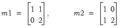
The commands,

create the matrices:

See “Matrix Language” for a detailed discussion of vector and matrix manipulation in EViews.

The freq command performs a one-way or N-way frequency tabulation.

Frequencies are computed for all of the rows of the matrix. Rows with NAs are dropped unless included by option. You may use options to control automatic binning (grouping) of values and the order of the entries of the table.

tabulates each value (no binning) of HRS in ascending order with counts, percentages, and cumulatives.

tabulates X including NAs. The values will be binned if INC has more than 200 distinct values; EViews will create at most 100 equal value-width bins. The number of bins may be less than 100.

displays tables of binned pairs of the first two columns of X for each bin/value of the remaining columns. The table will not contain row and column marginals.

displays the same table with the table rows and columns ordered from values with highest frequency to lowest.

See “One-Way Tabulation” and “N-Way Tabulation” for a discussion of frequency tables.

The syntax for reading Excel files is:

The following table_description elements may be used when reading Excel data:

The optional variables_description may be formed using the elements:

loads the active sheet of DATA.XLSX into the MATRIX_NAME matrix object.

reads the data contained in the “GDP data” sheet of “Data.XLS” into the MATRIX_NAME object.

The syntax for reading HTML pages is:

The following table_description elements may be used when reading an HTML file or page:

The optional variables_description may be formed using the elements:

loads into the MAT1 matrix object the data located in the HTML file “Data.HTML” located on the C:\ drive

loads into a matrix object MAT1 the data with the given URL located on the website site “http://www.tradingroom.com.au”. The column header is set to three rows.

The syntax for reading text or binary files is:

If a table_description is not provided, EViews will attempt to read the file as a free-format text file. The following table_description elements may be used when reading a text or binary file:

A central component of the table_description element is the format statement. You may specify the data format using the following table descriptors:

The optional variables_description may be formed using the elements:

reads “Data.CSV” into a MAT2, skipping the first 5 rows.

loads the comma delimited data “Date.TXT” into the MAT2 matrix object.

See also Matrix::export.

As a procedure, label changes the fields in the matrix label.

The first version of the command displays the label view of the matrix. The second version may be used to modify the label. Specify one of the following options along with optional text. If there is no text provided, the specified field will be cleared.

The following lines replace the remarks field of M1 with “Data from CPS 1988 March File”:

To append additional remarks to M1, and then to print the label view:

To clear and then set the units field, use:

See “Labeling Objects” for a discussion of labels.

See also Matrix::displayname.

saves the first three principal components (in normalized loadings form) to the workfile. The components will have variances that are proportional to the eigenvalues.

normalizes the scores so that the resulting series have variances that are equal to 1.

You may change the scaling for the normalized components so that the cross-products equal 1, using the cpnorm option:

See “Saving Component Scores” for further discussion. See Matrix::pcomp for tools to display the principal components results for the matrix.

The matrix keyword is followed by the name you wish to give the matrix. matrix also takes an optional argument specifying the row r and column c dimension of the matrix. Once declared, matrices may be resized by repeating the matrix command using the original name.

You may combine matrix declaration and assignment. If there is no assignment statement, the matrix will initially be filled with zeros.

You should use sym for symmetric matrices.

declares a matrix named MOM with one element, initialized to zero.

declares a 3 by 6 matrix named COEFS, filled with zeros.

See “Matrix Language” for further discussion.

See “Rowvector” and “Vector” and “Sym” for full descriptions of the various matrix objects.

See “Object Linking and Embedding (OLE)” for a discussion of using OLE with EViews.

There are two forms of the pcomp command. The first form, which applies when displaying eigenvalue table output or graphs of the ordered eigenvalues, has only options and no command argument.

The second form, which applies to the graphs of component loadings, component scores, and biplots, uses the optional argument to determine which components to plot. In this form:

where the [graph_list] is an optional list of integers and/or vectors containing integers identifying the components to plot. Multiple pairs are handled using the method specified in the “mult=” option.

If the list of component indices omitted, EViews will plot only first and second components. Note that the order of elements in the list matters; reversing the order of two indices reverses the axis on which each component is displayed.

stores the table view of the eigenvalues and eigenvectors of MAT1 in a table object named tab1, the eigenvalues in a vector named v1, and the eigenvectors in a matrix named m1.

displays the scree plot of the ordered eigenvalues computed from the covariance matrix.

displays a biplot where the scores are normalized to have variances that equal the eigenvalues of the Spearman correlation matrix computed for the series in MAT1.

See “Principal Components” for further discussion. See also “Covariance Analysis” for discussion of the preliminary computation.

Note that this view analyzes the eigenvalues and eigenvectors of a covariance (or other association) matrix computed from the series in a group or the columns of a matrix. You may use Sym::eigen to examine the eigenvalues of a symmetric matrix.

(This is a deprecated method of importing into a matrix. See Matrix::import for the currently supported method.)

May be used to import data into an existing workfile from a text, Excel, or Lotus file on disk.

You must supply the name of the source file. If you do not include the optional path specification, EViews will look for the file in the default directory. Path specifications may point to local or network drives. If the path specification contains a space, you may enclose the entire expression in double quotation marks.

If you do not specify the “t” option, EViews uses the file name extension to determine the file type. If you specify the “t” option, the file name extension will not be used to determine the file type.

reads data into matrix M1 from an ASCII file MYDAT.RAW in the A: drive. The data in the file are listed by row, and the missing value NA is coded as a “.” (dot or period).

reads data into matrix M1 from an Excel file CPS88 in the default directory. The data are organized by column (transposed), the upper left data cell is A2, and the data is read from a sheet named SHEET3.

reads the Excel file CPS91 into matrix M2 from the network drive specified in the path.

See “Importing Data” for a discussion and examples of importing data from external files.

See also Matrix::export.

You should follow the resample keyword and options with an output_name containing a name of the matrix to hold the output.

By default, EViews uses the output_name “*_b” so that “_b” will be appended to the name of the original matrix and used as the output name.

creates a new matrix F_RESAMPLE obtained by drawing 1000 rows with replacement from F.

will compute a weighted resample and save the results to the same sized matrix F_WEIGHTED. The rows in the source will be drawn with probabilities proportional to the corresponding values in the series WT. WT must have the same number of rows as F and must contain non-missing, non-negative values.

See “Resample” for a discussion of the resampling procedure. For additional discussion of wildcards, see Appendix A. “Wildcards”.

See also @resample and @permute for sampling from matrices.

resizes the matrix MAT1 to 3 rows and 5 columns, retaining the contents of any existing elements and initializing new elements to 0.

Sets the attribute attr to attr_value. Note that quoting the arguments may be required. Once added to an object, the attribute may be extracted using the @attr data member.

sets the “revised” attribute in the object A to the string “never”, and extracts the attribute into the string object S.

See “Adding Custom Attributes in the Label View” and “Adding Your Own Label Attributes”.

Follow the setcollabels command with a space delimited list of column labels. Note that each column label should not contain spaces unless it is enclosed in quotes. If you provide fewer labels than there are columns, EViews will keep the corresponding default column names (“C11”, “C12”, etc...).

sets the column label for the first column in matrix MAT1 to USA, the second to UK, and the third to FRANCE.

where format_arg is a set of arguments used to specify format settings. If necessary, you should enclose the format_arg in double quotes.

For matrices, setformat operates on all of the cells in the matrix.

To format numeric values, you should use one of the following format specifications:

To specify a format that groups digits into thousands using a comma separator, place a “t” after the format character. For example, to obtain a fixed number of decimal places with commas used to separate thousands, use “ft[.precision]”.

To use the period character to separate thousands and commas to denote decimal places, use “..” (two periods) when specifying the precision. For example, to obtain a fixed number of characters with a period used to separate thousands, use “ct[..precision]”.

If you wish to display negative numbers surrounded by parentheses (i.e., display the number -37.2 as “(37.2)”), you should enclose the format string in “()” (e.g., “f(.8)”).

To set the format for all cells in the matrix to fixed 5-digit precision, simply provide the format specification:

Other format specifications include:

See Matrix::setwidth, Matrix::setindent and Matrix::setjust for details on setting spreadsheet widths, indentation and justification.

where indent_arg is an indent value specified in 1/5 of a width unit. The width unit is computed from representative characters in the default font for the current spreadsheet (the EViews spreadsheet default font at the time the spreadsheet was created), and corresponds roughly to a single character. Indentation is only relevant for non-center justified cells.

The default value is taken from the Global Defaults at the time the spreadsheet view is created.

For matrices, setindent operates on all of the cells in the matrix.

To set the indentation for all the cells in a matrix object:

See Matrix::setwidth and Matrix::setjust for details on setting spreadsheet widths and justification.

where format_arg may be set to left, center, right, or auto (strings are left-justified and numbers are right-justified). Default display settings can be set in General Options; see “Spreadsheet Data Display”.

left-justifies the cells in the spreadsheet view of the matrix MAT1.

See Matrix::setwidth and Matrix::setindent for details on setting spreadsheet widths and indentation.

Follow the setrowlabels command with a space delimited list of row labels. Note that each row label should not contain spaces unless it is enclosed in quotes. If you provide fewer labels than there are rows, EViews will use the corresponding default row names (“R11”, “R12”, etc...).

sets the row label for the first row in matrix MAT1 to USA, the second to UK, and the third to FRANCE.

where width_arg specifies the width unit value. The width unit is computed from representative characters in the default font for the current spreadsheet (the EViews spreadsheet default font at the time the spreadsheet was created), and corresponds roughly to a single character. width_arg values may be non-integer values with resolution up to 1/10 of a width unit.

sets the width of all columns in matrix MAT1 to 12 width units.

See Matrix::setindent and Matrix::setjust for details on setting spreadsheet indentation and justification.

displays and prints the spreadsheet view of matrix MAT1.

where mode is either 0 or 1 where 0 displays the default row and column labels and 1 displays the custom row and column labels (if present).

displays the custom row and column labels for the M1 spreadsheet. If custom labels have not been set the default labels will be displayed.

displays the default row and column labels for the M1 spreadsheet.

See also Matrix::setcollabels and Matrix::setrowlabels.

Computes and displays a table of means, medians, maximum and minimum values, standard deviations, and other descriptive statistics for each column of the matrix.

The command

computes the descriptive statistics for each column of MATRIX1 after listwise deletion of rows with missing values. Alternately,

displays the descriptive statistics view of matrix1 showing the statistics for each column of the matrix computed using individual samples.

See “Descriptive Statistics” for a discussion of the descriptive statistics views of a group.

See also boxplot.

By default, testbtw will test for equality of means, but you may specify instead tests of medians or variances as an option, and choose whether to use balanced or unbalanced samples.

The commands

uses both parametric ANOVA and nonparametric approaches to test the equality of means of the two series WAGE_M and WAGE_F using individual samples to compute the means. Alternately, the command,

tests for equality of variances using a balanced sample after listwise deletion of rows with missing values.

See “Tests of Equality” for further discussion of these tests.

See also Series::testby and Series::teststat.

By default, testbtw will test for equality of means, but you may specify instead tests of medians or variances as an option, and choose whether to use balanced or unbalanced samples.

The command

uses both parametric ANOVA and nonparametric approaches to test the equality of the means of the columns of MAT1 using individual samples. Alternately, the command,

tests for equality of the column variances using a balanced sample after listwise deletion of rows with missing values.

See “Tests of Equality” for further discussion of these tests.

See also Series::testby and Series::teststat.

Creates a foreign format disk file containing EViews data. May be used to export EViews data to another program.

This routine should realistically only be used in the oft-hand chance that you wish to write into a Lotus file. Improved Excel, text, and other format writing is available in Matrix::export.

Follow the name of the matrix object by a period, the keyword, and the name for the output file. The optional path name may be on the local machine, or may point to a network drive. If the path name contains spaces, enclose the entire expression in double quotation marks. The entire matrix will be exported.

Note that EViews cannot, at present, write into an existing file. The file that you select will, if it exists, be replaced.

Options are specified in parentheses after the keyword and are used to specify the format of the output file.

If you omit the “t=” option, EViews will determine the type based on the file extension. Unrecognized extensions will be treated as ASCII files. For Lotus and Excel spreadsheet files specified without the “t=” option, EViews will automatically append the appropriate extension if it is not otherwise specified.

Writes the matrix M1 into an ASCII file named DAT1.CSV on the A: drive. NAs are coded as “.” (dot).

writes the same file in the default directory.

saves the contents of M1 in an Excel file “Results.xls” in the specified directory.

See “Exporting to a Spreadsheet or Text File” for a discussion.

See also Matrix::export, Matrix::read.