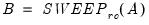
Function Reference: S
@scale Scale rows or columns of matrix.
@seas Seasonal dummy variable.
@second seconds of the minute of the observation.
@seq Vector containing arithmetic sequence.
@seqm Vector containing geometric sequence.
@sfill Create a string vector from a list of strings.
@sin Sine function in radians.
@skewsby Skewness for a series for each specified group.
@smape Symmetric mean absolute percentage error (difference) between series.
@sort Sort elements of data object.
@stdev Sample standard deviation (d.f. adjusted).
@stdevp Population standard deviation (no d.f. adjustment).
@stdevpsby Population standard deviations (d.f. corrected) for a series for each specified group.
@stdevs Sample standard deviation (d.f. adjusted).
@stdevsby Sample standard deviations (d.f. corrected) for a series for each specified group.
@stdevssby Sample standard deviations (d.f. corrected) for a series for each specified group.
@stdize Standardized data (using sample standard deviation).
@stdizep Standardized data (using population standard deviation).
@str String representation of number.
@strdate String corresponding to the date of the observation.
@stripcommas Remove leading and trailing commas surrounding string.
@stripparens Remove paired leading and trailing parentheses surrounding string.
@stripquotes Remove paired double-quotation marks surrounding string.
@strnow String representation of the current date and time.
@sumsby Sum of observations in a series for each specified group.
@sumsq Arithmetic sum of squares.
@sumsqsby Sum of squared observations in a series for each specified group.
@svd Singular value decomposition (economy) of matrix.
@svdfull Singular value decomposition (full) of matrix.
Scale rows or columns of matrix.
Syntax: @scale(m, v[,p])
m: matrix, sym
v: vector
p: (optional) number
Return: matrix or sym
Scale the rows or columns of a matrix, or the rows and columns of a sym matrix.
• If m is a matrix and v is a vector, the i-th row of m will be scaled by the i-th element of v, optionally raised to the power p (row scaling). The length v must equal the number of rows of m.
• If m is a matrix and v is a rowvector, the i-th column of m will be scaled by the i-th element of v, optionally raised to the power p (column scaling). The length v must equal the number of columns of m.
• If m is a sym object, then v may either be a vector or a rowvector. The (i,j)-th element of m will be scaled by both the i-th and j-th elements of v (row and column scaling). The length v must equal the number of rows (and columns) of m.
Let M be the matrix object, V be the vector or rowvector, and
be the diagonal matrix formed from the elements of V. Then
@scale(m, v, p) returns:
• 
, if M is a matrix and V is a vector.
• 
, if M is a matrix and V is a rowvector.
• 
, if M is a sym matrix.
Examples
sym covmat = @cov(grp1)
vector vars = @getmaindiagonal(covmat)
sym corrmat = @scale(covmat, vars, -0.5)
computes the covariance matrix for the series in the group object GRP1, extracts the variances to a vector VARS, then uses VARS to obtain a correlation matrix from the covariance matrix.
Cross-references
Seasonal dummy variable.
Syntax: @seas(x)
x: integer
Return: series
Returns the seasonal dummy variable series in a quarterly or monthly workfile, indicating whether the date in the workfile of each observation matches the seasonal value specified in x.
Examples
workfile m 2020 2022
series m2 = @seas(2)
creates a dummy variable series with February observations (seasonal 2) equal to 1.
workfile q 2020 2021
smpl if @seas(2) = 1
creates a quarterly workfile, then sets the sample to include only observations in the second quarter.
Cross-references
Seconds of the minute of the observation.
Syntax: @second
Return: series
Returns the seconds of the minute (0–59) associated with each observation in the workfile.
• If the workfile is of lower than second frequency, all observations will be set to 0.
• If the workfile is undated, observations will be set to -1.
Examples
series dt = @second
saves the seconds of the minute into the series DT.
The command
smpl if @second = 59
sets the sample to only include observations for the last second of the minute.
Cross-references
Vector containing arithmetic sequence.
Syntax: @seq(d1, d2, n)
d1: number
d2: number
n: integer
Return: vector
Returns a vector holding an arithmetic sequence of n elements. The initial element has value d1, and the difference between each element and its predecessor is d2.
Examples
vector v1 = @seq(0, 1/3, 10)
creates V1, a 10-element vector with first element 0, and each subsequent element increasing by 1/3.
vector cdf1 = @cnorm(@seq(-2.0, 0.01, 401))
create a 401-element vector of values of the normal CDF evaluated at points from -2.0 to 2.0
Cross-references
See also
@grid,
@range, and
@seqm.
Vector containing geometric sequence.
Syntax: @seqm(d1, d2, n)
d1: number
d2: number
n: integer
Return: vector
Returns a vector holding a geometric sequence of n elements. The initial element has value d1, and the ratio between each subsequent element and its predecessor is d2.
Examples
vector v1 = @seqm(1, 2, 10)
creates a V1, a 10-element vector with first element 1, and each subsequent element representing a power of 2.
Cross-references
See also
@grid,
@range, and
@seq.
Create a string vector from a list of strings.
Syntax: @sfill(str1[, str2, str3, ...])
str1: string
strs: string str2, str3, ...
Return: svector
Returns an svector containing strings specified in a comma separated list of strings.
Examples
If string list SS01 contains “A B C D E F”, then
svector s1 = @sfill("A", "B", "C", "D", "E", "F")
returns the 6 element svector S1, where row one of S1 contains “A”, row two contains “B”, etc.
svector s2 = @sfill("my apples", "your oranges", "our pears")
creates a 3 element svector S2, with the rows containing “my apples”, “your oranges”, and “our pears”.
Cross-references
See also
@wsplit. See
@wjoin for obtaining a string from an svector.
Sign of number.
Syntax: @sign(x)
x: number
Return: integer
Returns sign of x: -1, 0, 1 depending on the sign of x (“<0”, “=0”, “>0”).
Examples
= @sign(1.23)
returns 1.
matrix m1 = @round(@mnrnd(30, 2))
matrix m2 = @sign(m1)
produces a

matrix of -1, 0, and 1 depending on the sign of the corresponding element of the randomly generated matrix M1.
vector v1 = @round(@mnrnd(30))
vector v2 = @sign(v1)
produces a

-element sign vector corresponding to V1.
Cross-references
See also
@egt,
@eeq, and
@elt.
Sine function in radians.
Compute the sine of x (specified in radians).
Syntax: @asin(x)
x: number
Return: number
Examples
= @sin(@pi/2)
returns 1.
Cross-references
Skewness.
Computes the skewness of the elements of x.
Syntax: @skew(x[, s])
x: series, vector, matrix
s: (optional) sample string or object when x is a series and assigning to a series
Return: number
The skewness is calculated as
where

is the sample mean, and

is an estimator for the standard deviation that is based on the biased estimator for the variance
The skewness of a symmetric distribution, such as the normal distribution, is zero. Positive skewness means that the distribution has a long right tail and negative skewness implies that the distribution has a long left tail.
For series calculations, EViews will use the current or specified workfile sample.
Examples
If x = @nrnd, then
= @skew(x)
returns a value close to 0 in large samples (since the normal distribution is symmetric).
Cross-references
See also
@mean,
@var, and
@kurt.
Skewness for a series for each specified group.
Syntax: @skewsby(x, y[y1, y2, ... yn, s])
x: series
y: series, alpha
s: (optional) sample string or object
Return: series
Returns the skewnesses of x for each group defined by distinct values of y.
EViews will use the current or specified workfile sample.
Examples
show @skewsby(x, g1, g2)
produces a linked series of the by-group sample skews of the series x, where members of the same group have identical values for both g1 and g2.
Cross-references
See also
@skew and
@kurtsby.
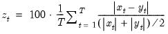
Symmetric mean absolute percentage error (difference) between series.
Computes the mean of the symmetric absolute percentage difference between x and y.
Syntax: @smape(x, y, [s])
x: series
y: series
s: (optional) sample string or object
Return: number
EViews will use the current or specified workfile sample.
Examples
Let yf denote in-sample forecasts for the series y. Then
= @smape(yf, y)
returns the SMAPE between the series y and its forecast.
Cross-references
Solve system of linear equations.
Syntax: @solvesystem(o, v)
m: matrix, sym
v: vector
Return: vector
Returns the vector
x that solves the linear system

where the matrix or sym

is given by the argument
m, and the vector is given by the argument
v.Examples
We first create a workfile, generate a random series, and create a group for estimating a trend regression.
workfile u 100
series y = nrnd
group g 1 @trend
We extract the moment matrices,
matrix xx = @inner(g)
vector xy = @transpose(@convert(g)) * @convert(y)
and solve the moment conditions to obtain regression coefficient estimates
vector b1 = @solvesystem(xx, xy)
We may compare these results to those obtained by estimation using series and the equation object:
equation eq1.ls y g
vector b2 = eq1.@coefs
and see that B1 and B2 are identical.
Cross-references
Sort elements of matrix or vector.
Syntax: @sort(m[, o])
m: matrix or vector
o: (optional) string
Return: matrix, vector
Returns a matrix or vector containing the sorted elements of the matrix or vector object m.
Note that sorting a matrix ranks every element of the matrix and arranges the results to match the elements of the original matrix, from upper left to lower right.
The o option controls the direction of the ranking:
• “a” (ascending - default) or “d” (descending)
Examples
Let M1 be an

matrix. Then
= @sort(m1, "d")
returns an

matrix whose elements are those of M1, sorted from largest to smallest in column-major order.
Cross-references
Square root.
Syntax: sqr(x)
x: number
Return: number
Returns the square root, for x > 0.
Examples
= sqr(9)
returns 3.
Cross-references
Square root.
Syntax: @sqrt(x)
x: number
Return: number
Returns the square root, for x > 0.
Examples
= @sqrt(9)
returns 3.
Cross-references
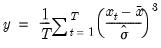
Sample standard deviation (d.f. adjusted).
Square root of sample (d.f. adjusted) Pearson product moment variance.
Syntax: @stdev(x, [s])
x: series, vector, matrix
s: (optional) sample string or object when x is a series and assigning to a series
Return: number
The sample standard deviation is calculated as
where

is the mean of

.
For series calculations, EViews will use the current or specified workfile sample.
Examples
If x = @nrnd, then
= @stdev(x)
returns a value near 1 in large samples.
Cross-references
See also
@stdevp,
@stdevs, and
@var.
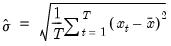
Population standard deviation (no d.f. adjustment).
Square root of population (non-d.f. adjusted) Pearson product moment variance.
Syntax: @stdevp(x, [s])
x: series, vector, matrix
s: (optional) sample string or object when x is a series and assigning to a series
Return: number
The population standard deviation is calculated as
where

is the mean of

.
For series calculations, EViews will use the current or specified workfile sample.
Examples
If x = @nrnd, then
= @stdevp(x)
returns a value near 1 in large samples.
Cross-references
See also
@stdev,
@stdevs, and
@varp.
Population standard deviations (d.f. corrected) for a series for each specified group.
Syntax: @stdevspby(x, y[y1, y2, ... yn, s])
x: series
y series, alpha
s: (optional) sample string or object
Return: series
Returns the population Pearson product moment standard deviations (d.f. corrected) for x each group defined by distinct values of y.
EViews will use the current or specified workfile sample.
Examples
show @stdevpsby(x, g1, g2)
produces a linked series of the by-group population standard deviations of the series x, where members of the same group have identical values for both g1 and g2.
Cross-references
Sample standard deviation (d.f. adjustment).
Square root of sample (d.f. adjusted) Pearson product moment variance.
Syntax: @stdevs(x, [s])
x: series, vector, matrix
s: (optional) sample string or object when x is a series and assigning to a series
Return: number
Equivalent to @stdev.
For series calculations, EViews will use the current or specified workfile sample.
Examples
x = @nrnd
= @stdevs(x)
returns a value near 1 in large samples.
Cross-references
See also
@stdev,
@stdevp, and
@vars.
Sample standard deviations (d.f. corrected) for a series for each specified group.
Syntax: @stdevsby(x, y[y1, y2, ... yn, s])
x: series
y series, alpha
s: (optional) sample string or object
Return: series
Returns the sample standard deviations (d.f. corrected) for x each group defined by distinct values of y.
EViews will use the current or specified workfile sample.
Examples
show @stdevsby(x, g1, g2)
produces a linked series of the by-group sample standard deviations of the series x, where members of the same group have identical values for both g1 and g2.
Cross-references
Sample standard deviations (d.f. corrected) for a series for each specified group.
Syntax: @stdevssby(x, y[y1, y2, ... yn, s])
x: series
y series, alpha
s: (optional) sample string or object
Return: series
Returns the Pearson product moment sample standard deviations (d.f. corrected) for x each group defined by distinct values of y.
EViews will use the current or specified workfile sample.
Examples
show @stdevssby(x, g1, g2)
produces a linked series of the by-group sample standard deviations of the series x, where members of the same group have identical values for both g1 and g2.
Consider the commands
matrix m = @mrnd(100,100)
@mean(m)
@vars(m)
matrix stdm = @stdize(m)
@mean(stdm)
@vars(stdm)
The matrix M should have mean approximately 0.5 and sample variance approximately 0.083. The standardized matrix, STDM, should have mean approximately 0 and sample variance of 1.
Cross-references
Standardized data (using sample standard deviation).
Return copy of data scaled and translated to have a mean of zero and a Pearson product moment sample standard deviation of one.
Syntax: @stdize(x, [s])
x: series, vector, matrix
s: (optional) sample string or object when x is a series and assigning to a series
Return: series, vector, matrix object
The adjusted data are calculated as
where

and

are the mean and sample standard deviation, respectively, of

.
For series calculations, EViews will use the current or specified workfile sample.
Examples
show @stdize(x)
returns a linked series of the standardized values of x.
Consider the commands
matrix m = @mrnd(100,100)
@mean(m)
@varp(m)
matrix stdm = @stdizep(m)
@mean(stdm)
@varp(stdm)
The matrix M should have mean approximately 0.5 and population variance approximately 0.083. The standardized matrix, STDM, should have mean approximately 0 and population variance of 1.
Cross-references
Standardized data (using population standard deviation).
Return copy of data scaled and translated to have a mean of zero and a population (non-d.f. adjusted) Pearson product moment standard deviation of one.
Syntax: @stdizep(x, [s])
x: series, vector, matrix
s: (optional) sample string or object when x is a series and assigning to a series
Return: series, vector, matrix object
The adjusted data are calculated as
where

and

are the mean and population standard deviation, respectively, of

.
For series calculations, EViews will use the current or specified workfile sample.
Examples
show @stdize(x)
returns a linked series of the standardized values of x.
Consider the commands
matrix m = @mrnd(100,100)
@mean(m)
@varp(m)
matrix stdm = @stdizep(m)
@mean(stdm)
@varp(stdm)
The matrix M should have mean approximately 0.5 and population variance approximately 0.083. The standardized matrix, STDM, should have mean approximately 0 and population variance of 1.
Cross-references
String representation of number.
Syntax: @str(d[, fmt])
d: number
fmt: (optional) numeric format string
Return: string
Returns a string representing in d. You may provide an optional format string, fmt.
By default, EViews will format the number string using 10 significant digits, with no leading or trailing characters, no thousands separators, and an explicit decimal point.
(The default conversion is equivalent to using @str with the format “g.10” as described below.)
You may provide an explicit format string fmt to write your number in a specific fashion. A numeric format string has the format:
[type][t][+][(][$][#][<|=|>][0][width][[.|..]precision][%][)]
There are a large number of syntax elements in this format but we may simplify matters greatly by dividing them into four basic categories:
• format: [type]
• width: [<|=|>][width]
• precision: [precision]
• advanced modifiers: the remaining elements (leading and trailing characters, padding and truncation modifiers, separators, display of negative numbers)
The
type,
width, and
precision components are the basic components of the format so we will focus on them first. We describe the advanced modifiers in
“Modified Formats”.
Basic Formats
EViews offers formats designed for both real-valued and integer data.
Basic Real-Value Formats
The basic real-value format is:
[type][<|=|>][width][.][precision]
The
type component is a single character indicating the basic type and the
width and
precision arguments are numbers indicating the number of output characters and the precision at which the numbers should be written. If specified, the precision should be separated from the
type and width portion of the format by a “.” character (or “..” as we will see in
“Modified Formats”).
If you specify a format with neither width nor precision, EViews will format the number at full precision with matching string width.
The following types are for use with real-valued data:
g | significant digits |
z | significant digits with trailing zeros |
c | fixed characters with single leading space for positive numbers |
f | fixed decimal places |
e | scientific/float |
p | percentage (same as “f” but values are multiplied by 100) |
s | suppressed decimal point format |
r | ratio, e.g., “30 1/5” |
The type character may be followed by a width specification, consisting of a width indicating the number of output characters, optionally preceded by a “>”, “=” or “<” modifier.
• If no width is provided, the number will be rendered in a string of the exact length required to represent the value (e.g., the number 1.23450 will return “1.2345”, a string of length 6).
• If an unmodified
width or one with the “>” modifier is provided, the specified number places a
lower-bound on the width of the string: the output will be left-padded to the specified width, if necessary, otherwise the string will be lengthened to accommodate the full output. By default, padding will use spaces, but you may elect to use 0’s by providing an advanced modifier (
“Modified Formats”).
• If the“<” modifier is provided along with width, the width places an upper-bound on the width of the string: the output will not be padded to the specified width. If the number of output characters exceeds the width, EViews will return a width-length string filled with the “#” character.
• If the“=” modifier is provided along with width, the width provides an exact-bound for the width of the string: the output will be padded to specified width, if necessary. If the number of characters exceeds the width, EViews will return a width-length string filled with the “#” character.
If you specify a precision, the interpretation of the value will vary depending on the format type. For example, precision represents the number of significant digits in the “g” and “z” formats, the number of characters in the “c” format, and the number of digits to the right of the decimal in the “f”, “e”, “p”, and “s” formats. For the “r” format, the precision determines maximum denominator for the fractional portion (as a power-of-10).
The following guidelines are used to determine the precision implied by a number format:
• If you specify a format with only a precision specification, the precision will implicitly determine the width at which your numbers are written.
• If you specify a format with only a width specification, the width will implicitly determine the precision at which your numbers are written. Bear in mind that only the modified width specifications “=width” and “<width” impose binding restrictions on the precision.
• If you specify a format using both width and precision, the precision at which your numbers are written will be determined by whichever setting is most restrictive (i.e., “f=4.8” and “f=4.2” both imply a formatted number with two digits to the right of the decimal).)
Basic Integer Formats
The basic integer format is:
[type][<|=|>][width]
The type component is a single character indicating the basic type. The following types are for use with integer data:
i | integer |
h | hexadecimal |
o | octal |
b | binary |
If one of the integer formats is used with real-valued data, the non-integer portion of the number will be ignored. You may specify a
width using the syntax and rules described in
“Basic Real-Value Formats”.
Modified Formats
Recall that the syntax of a numeric format string is given by:
[type][t][+][(][$][#][<|=|>][0][width][[.|..]precision][%][)]
In addition to the basic type, width, and precision specifiers, the formats take a set of modifiers which provide you with additional control over the appearance of your output string:
• You may combine any of the real-value format characters (“g”, “e”, “f”, etc.) with the letter “t” (“gt”, “et”, “ft”, etc.) to display a thousands separator (“1,234.56”). By default, the separator will be a comma “,”, but the character may be changed to a “.” using the “..” format as described below.
• You may add a “+” symbol after the format character (“g+”, “et+”, “i+”) to display positive numbers with a leading “+”.
• To display negative numbers within parentheses, you should enclose the remaining portion of the format in parentheses “ft+($8.2)”.
• Add “$” to the format to display a leading “$” currency character.
• You should include a “#” to display a trailing point in scientific notation (e.g., “3.e+34”).
• The width argument should include a leading zero (“0”) if you wish padded numbers to display leading zeros instead of spaces (“g08.2”, “i05”).
• If you added a “t” character to your real-value format type, you may replace the usual “.” width-precision separator with “..” (“ft<08..2”, “e=7..”, “g..9”, etc.) to reverse the thousands and decimal separators so that thousands will be separated by a “.” and decimal portion by a “,” (“1.234,56”).
• Adding a “%” character to the end of the format adds the “%” character to the end of the resulting string.
Examples
string num = @str(1.23)
assigns to the string NUM the text “1.23”.
alpha alpha1 = @str(-123.88)
assigns the string “-123.88” to the alpha series ALPHA1.
string num = @str(123456,"z.9")
returns a string formatted to 9 significant digits with trailing zeros: “123456.000”.
string num = @str(123456,"z.4")
returns a string formatted to 4 significant digits with trailing zeros: “1.235e+05”. Note that since the input number has more than 4 significant digits, no trailing zeros are added and the resulting string is identical to one that would have been produced with a “g.4” format.
string num = @str(126.543,"c.7%")
returns a string with exactly 7 characters, including a leading space, and a trailing percent sign: “ 126.5%”.
string num = @str(126.543,"p.7")
converts the number 126.543 into a percentage with 7 decimal places and returns “12654.3000000”. Note no percent sign is included in the string.
string num = @str(1.83542,"f$5.4")
returns “$1.8354”. The width selection of “5” with an implicit “>” modifier is irrelevant, since the precision setting of “4”, coupled with the insertion of the “$” symbol yields a string with more characters than “5”.
string num = @str(1.83542,"f$8.4")
returns “ $1.8354”. Here the width selection is binding, and a leading space has been added to the string.
string num = @str(1.83542,"f$=5.4")
returns “ $1.84”. The explicit “=” width modifier causes the width setting of “5” to be binding.
string num = @str(524.784,"r")
converts the number 524.784 into a ratio representation: “524 98/125”.
string num = @str(1784.321,"r=3")
will return “###”, since there is no way to represent 1784.321 as a string with only 3 characters.
string num = @str(543,"b")
converts the number 543 into a binary representation: “1000011111”.
The matrix command
svector svec1 = @str(v1)
converts the numeric values of vector V1 to strings and puts the results in the svector SVEC1. If the svector SVEC1 exists it will be sized to match the rows of V1 and missing values will be converted to empty strings.
The series command
alpha a1 = @val(gdp)
creates the alpha series A1 and converts the numeric values of series GDP to string. NA values will be become empty strings.
Format strings may be used to govern the conversion,
svector svbin = @str(vec1, "e")
converts the numeric values in the vector VEC1 into their strings representation in scientific notation and assigns them to the svector SVBIN.
Cross-references
See
@val to interpret strings as numbers.
String representation of the dates of the observation.
Syntax: @strdate(fmt)
fmt: date format string
Return: alpha
Fill an alpha series with workfile dates as strings, using the date format string fmt, for each observation in the workfile sample. Only observations in the workfile sample will be filled.
Date format syntax is outlined in
“Date Formats”.
@strdate is a specialized form of a call to the
@datestr function, applied to all of the observations in the workfile.
Examples
The commands
alpha wfdates1 = @strdate("yyyy/mm/dd")
alpha wfdates2 = @datestr(@date, "yyyy/mm/dd")
fill the alpha series WFDATES1 and WFDATES2 with the corresponding workfile dates in “yyyy/mm/dd” format.
alpha hmsdates = @strdate("yyyy-MM-DD HH:mi:ss")
fills the alpha series HMSDATES with the workfile dates in "yyyy-MM-DD HH:mi:ss" format.
Cross-references
See
@datestr and
@strnow for other functions to obtain date strings.
See
@dateval for converting date strings to date numbers.
Remove leading and trailing commas surrounding string.
Syntax: @stripcommas(str)
str: string
Return: string
Returns the contents of the string str with leading and trailing commas (ignoring whitespace) stripped.
Leading and trailing commas are always removed, even if unpaired. All whitespace characters up to the leading comma and whitespace characters after the trailing comma are also removed.
Examples
Define the string object
string s1 = " , lettuce, tomato, onion, "
so that S1 contains the string “ , lettuce, tomato, onion, ”. Note the presence of the whitespace before the leading, and after the trailing comma.
Then the commands
string sc1 = @stripcommas(" , lettuce, tomato, onion, ")
string sc2 = @stripcommas(s1)
create SC1 and SC2 which contain the string “ lettuce, tomato, onion”. Note that the resulting string retains the space (“ ”) after the initial comma, but not the space after the last comma in S1.
If ALPHA1 is an alpha series, the command
alpha a1 = @stripcommas(alpha1)
fills A1 with strip-comma values of ALPHA1 for each observation in the workfile sample.
If AVEC1 is an svector, the commands
svector as1 = @stripcommas(avec1)
svector as2 = @stripcommas(avec1.@rows(@fill(1, 3, 5))
create svectors AS1 and AS2, where AS1 contains double-quoted values of AVEC1, and AS2 contains double-quoted values of the rows 1, 3, and 5 of AVEC1.
Cross-references
Remove paired leading and trailing parentheses surrounding string.
Syntax: @stripparens(str)
str: string
Return: string
Returns the contents of the string str with parentheses (“( )”) stripped from both the left and the right ends. If a parenthesis is present on only the left or right end, the parenthesis will be retained.
Examples
Let
string s1 = "(I don’t know)"
so that S1 contains the string “(I don’t know)”.
Then the commands
string sq1 = @stripparens("(I don’t know)")
string sq2 = @stripparens(s1)
create SQ1 and SQ2 which contain the string “I don’t know”.
If ALPHA1 is an alpha series, the command
alpha a1 = @stripquotes(alpha1)
fills A1 with parens-removed values of ALPHA1 for each observation in the workfile sample.
If AVEC1 is an svector, the commands
svector as1 = @stripparens(avec1)
svector as2 = @stripparens(avec1.@rows(@range(2, 6))
creates svectors AS1 and AS2, where AS1 contains parens-removed values of AVEC1, and AS2 contains parens-removed values of the rows 2 through 6 of AVEC1.
Cross-references
Remove paired double-quotation marks surrounding string.
Syntax: @stripquotes(str)
str: string
Return: string
Returns the contents of the string str with double-quotation marks stripped from both the left and the right ends with leading and trailing whitespace ignored. If a double-quote is present on only the left or right end, the double-quote will be retained.
Examples
Let
string s1 = """Chicken Marsala"""
so that S1 contains the quoted string “"Chicken Marsala"”.
Then the commands
string sq1 = @stripquotes("""Chicken Marsala""")
string sq2 = @stripquotes(s1)
create SQ1 and SQ2 which contain the un-quoted string “Chicken Marsala”.
If ALPHA1 is an alpha series, the command
alpha a1 = @stripquotes(alpha1)
fills A1 with strip-quoted values of ALPHA1 for each observation in the workfile sample.
If AVEC1 is an svector, the commands
svector as1 = @stripquotes(avec1)
svector as2 = @stripquotes(avec1.@rows(@fill(1, 3, 5))
create svectors AS1 and AS2, where AS1 contains double-quoted values of AVEC1, and AS2 contains double-quoted values of the rows 1, 3, and 5 of AVEC1.
Cross-references
Length of string.
Syntax: (str)
str: string
Return: integer
Returns the length of the string str.
Examples
Let
string s1 = "(I don’t know)"
so that S1 contains the string “(I don’t know)”.
Then the commands
@strlen("(I don’t know)")
@strlen(s1)
both return the scalar value 14.
If ALPHA1 is an alpha series, the command
series d1 = @strlen(alpha1)
fills D1 with lengths of the strings in ALPHA1 for each observation in the workfile sample.
If AVEC1 is an svector, the commands
vector vec1 = @strlen(avec1)
creates the vector VEC1 containing the lengths of the elements of AVEC1.
Cross-references
String representation of the current date and time.
Syntax: @strnow(fmt)
fmt: date format string
Return: string
Returns a string representation of the current date number (at the moment the function is evaluated) using the date format string, fmt.
Date format syntax is outlined in
“Date Formats”.
Exampless
The command
@strnow("DD/mm/yyyy")
@datestr(@now, "DD/mm/yyyy")
both return the dates string at the moment of evaluation in “DD/mm/yyyy” format.
Using intra-day formats,
@strnow("yyyy-MM-DD HH:mi:ss")
@datestr(@now, "yyyy-MM-DD HH:mi:ss")
both return the date string at the moment of evaluation in "yyyy-MM-DD HH:mi:ss" format.
Cross-references
Extract submatrix from matrix object.
Syntax: @subextract(m, n1, n2[, n3, n4])
m: matrix, vector, sym
n1: integer
n2: integer
n3: (optional) integer
n4: (optional) integer
Return: matrix
Returns a submatrix of a specified matrix, m.
• The required arguments n1 and n2 are the row and column of the upper left corner of the region to be extracted.
• The optional arguments n3 and n4 provide the row and column of the lower right corner of the region to be extracted.
• If n3 or n4 are not provided, the corresponding element will be the last row or column of the source matrix.
Note that in some circumstances, you may find it easier to use the newer “.sub”, “.row”, and “.col” object data member functions. See
“Matrix Data Members” and
“Sym Data Members” and the examples below.
Examples
matrix m1 = @mnrnd(20, 5)
matrix m1a = @subextract(m1, 3, 2)
extracts the

matrix from the lower right corner of M1 starting at row 3 and column 2, while
matrix m1b = @subextract(m1, 1, 1, 5, 4)
extracts the upper left corner of M2 up through row 5 and column 4.
matrix m1c = @subextract(m1, 3, 2, 7, 3)
extracts the subtract from rows 3 to 7 and columns 2 to 3.
The commands
matrix m1d = @subextract(m1, 3, 1, 3)
rowvector v1d = @rowextract(m1, 3)
both extract row 3 from the matrix, while
matrix m1e = @subextract(m1, 1, 4, @rows(m1), 4)
vector v1e = @columnextract(m1, 4)
extract column 4.
For illustration purposes, we repeat the previous commands followed by data member functions to perform equivalent extractions:
• lower corner extraction,
matrix m1a = @subextract(m1, 3, 2)
matrix m1a_1 = m1.@sub(@range(3, m1.@rows), @range(2, m1.@cols))
• upper corner extraction,
matrix m1b = @subextract(m1, 1, 1, 5, 4)
matrix m1b_1 = m1.@sub(@range(1, 5), @range(1, 4))
• arbitrary rectangle extraction
matrix m1c = @subextract(m1, 3, 2, 7, 4)
matrix m1c_1 = m1.@sub(@range(3, 7), @range(2, 4))
• row extraction as rowvector
matrix m1d = @subextract(m1, 3, 1, 3)
matrix m1d_1 = m1.@sub(3, @range(1, m1.@cols))
rowvector v1d = @rowextract(m1, 3)
rowvector v1d_1 = @transpose(m1.@row(3))
• column extraction
matrix m1e = @subextract(m1, 1, 4, @rows(m1), 4)
matrix m1e_1 = m1.@sub(@range(1, @rows(m1)), 4)
vector v1e = @columnextract(m1, 4)
vector v1e_1 = m1.@col(4)
Cross-references
Arithmetic sum.
Computes the sum of the elements of x.
Syntax: @sum(x[, s])
x: series, vector, matrix
s: (optional) sample string or object when x is a series and assigning to a series
Return: number
For series calculations, EViews will use the current or specified workfile sample.
Examples
If x is a series of length 5 whose elements are 1, 2, 3, 4, 5, then
= @sum(x)
returns 15.
Cross-references
See also
@inner,
@prod, and
@sumsq.
Sum of observations in a series for each specified group.
Syntax: @sumsby(x, y[y1, y2, ... yn, s])
x: series
y series, alpha
s: (optional) sample string or object
Return: series
Compute the sum of observations in x for group identifiers defined by distinct values of y.
EViews will use the current or specified workfile sample.
Examples
show @sumsby(x, g1, g2)
produces a linked series of by-group sums of observations in x, where members of the same group have identical values for both g1 and g2.
Cross-references
Arithmetic sum of squares.
Computes the sum of the squared elements of x.
Syntax: @sumsq(x[, s])
x: series, vector, matrix
s: (optional) sample string or object when x is a series and assigning to a series
Return: number
For series calculations, EViews will use the current or specified workfile sample.
Examples
If x is a series of length 5 whose elements are 1, 2, 3, 4, 5, then
= @sumsq(x)
returns 55.
Cross-references
See also
@inner,
@prod, and
@sum.
Sum of squared observations in a series for each specified group.
Syntax: @sumsqsby(x, y, [s])
x: series
y series, alpha
s: (optional) sample string or object
Return: series
Compute the sum of squared observations in x for group identifiers defined by distinct values of y.
EViews will use the current or specified workfile sample.
Examples
show @sumsqsby(x, g1, g2)
produces a linked series of by-group sums of squares of observations in x, where members of the same group have identical values for both g1 and g2.
Cross-references
Singular value decomposition (economy) of matrix
Syntax: @svd(m1, v1, m2)
m1: matrix, sym
v1: vector

m2: matrix, sym

Return: matrix

Performs an “economy” or “thin” singular value decomposition of the matrix m1, generating truncated results when m1 is not square (exploiting the reduced maximum rank of a non-square matrix).
The matrix

is returned by the function, the vector
v1 will be filled (resized if necessary) with the singular values and the matrix
m2 will be assigned (resized if necessary) the other matrix,

, of the decomposition. The singular value decomposition satisfies:
where

is a diagonal matrix with the singular values along the diagonal. Singular values close to zero indicate that the matrix may not be of full rank. See the
@rank function for a related discussion.
Let r be the number of rows of m1 and s be the number of columns of m1 so that m1 has at most t = min(r, s) distinct singular values. Then
• m2 will be s-by-t
• v1 will be t-by-1
• 
will have dimensions
r-by-
t Examples
matrix x = @mnrnd(5, 7)
vector w
matrix v
matrix u = @svd(x, w, v)
performs the thin SVD of the matrix X. U is

, W is a 5 element vector containing the singular values, and V is a

matrix.
Alternately, if the rank is less than the number of rows,
matrix x = @mnrnd(7, 5)
matrix u = @svd(x, w, v)
U is

, W is a 5 element vector containing the singular values, and V is a

matrix.
The following demonstrate the properties of the decomposition:
sym i1 = @inner(u)
sym i2 = @inner(v)
matrix x1 = u * @makediagonal(w) * v.@t
where I1 and I2 and the identity matrix, and X1 is equal to X.
Cross-references
Singular value decomposition (full) of matrix
Syntax: @svdfull(m1, m2, m3)
m1: matrix, sym
m2: matrix
m3: matrix, sym
Return: matrix
Performs a singular value decomposition of the matrix m1.
The matrix

is returned by the function, the matrix
m2 will be assigned (resized if necessary) the matrix

, and the matrix
m3 will be assigned (resized if necessary) the other matrix,

, of the decomposition. The singular value decomposition satisfies:
where

is a diagonal matrix with the singular values along the diagonal. Singular values close to zero indicate that the matrix may not be of full rank. See the
@rank function for a related discussion.
Examples
matrix x = @mnrnd(5, 7)
matrix w
matrix v
matrix u = @svdfull(x, w, v)
performs the full SVD of the matrix X. U is

, W is

diagonal matrix with singular values on the diagonal, and V is

.
Alternately, if the rank is less than the number of rows,
matrix x = @mnrnd(7, 5)
matrix u = @svdfull(x, w, v)
then U is

, W is a

matrix with the singular values on the main diagonal and V is a

matrix.
In both cases, the following demonstrate the properties of the decomposition:
sym i1 = @inner(u)
sym i2 = @inner(v)
matrix x1 = u * w * v.@t
where I1 and I2 and the identity matrix, and X1 is equal to X.
Cross-references
See also
@svd,
@cholesky,
@lu, and
@qr.
Sweep operator.
There are two syntaxes for @sweep, one for the symmetric, and the other for then non-symmetric operator.
Syntax: @sweep(s[, n])
s: sym
k: integer
k2: (optional) integer
Return: matrix
Returns the result of applying the symmetric sweep operator to symmetric matrix S at diagonal element k. If k2 is specified, sweeps on all diagonal elements between k and k2, inclusive.
Syntax: @sweep(m, r, c)
m: matrix, sym
r: integer
c: integer
Return: matrix
Returns the result of applying the non-symmetric sweep operator to general matrix m at element (r, c).
The sweep operator is an elementary matrix row operation with particularly useful properties when applied to uncorrected sum of squares and cross-products (USSCP) matrices. Among these properties is the ability to calculate the coefficients for one or more regressions over a common set of regressors.
Let
be an application of the symmetric sweep operator. Then,
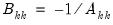
,
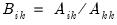
where

,
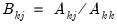
where

, and
where

and

.
Let
be an application of the non-symmetric sweep operator. Then,
,
where

,
where

, and
where

and

.
Examples
As an example of using the sweep operator to replicate the results of OLS regression, suppose we have series for one dependent variable, Y, and three regressors, X1, X2, X3.
We can organize the data into a group YX = [Y X1 X2 X3], form the USSCP matrix (YX)'YX, and apply the sweep operator to the three diagonal elements associated with the regressors (elements 2-4).
Each application of the sweep operator to a diagonal element effectively switches the role of the associated variable from dependent to regressor.
workfile u 1000
series y = nrnd
series x1 = nrnd
series x2 = nrnd
series x3 = nrnd
group g y x1 x2 x3
sym usscp = @inner(g)
sym S = @sweep(usscp, 2, 4)
The resulting block matrix will have the form:
This matrix contains all the information usually associated with the results of OLS regression, which we can extract.
vector beta = @subextract(S, 2, 1, 4, 1) ' Regressor coefficients
scalar SSR = S(1,1) ' Sum of squared residuals
sym invXtX = -@subextract(S, 2, 2)
vector se = @sqrt(SSR * @getmaindiagonal(invXtX) / (@obssmpl - 3)) ' Coefficient standard errors
We could compare these results to those of a standard equation object for the same regression.
equation eq.ls(noconst) y x1 x2 x3
It is also possible to conduct multiple regressions against a set of common regressors. Consider a small example with two dependent variables, y1 and y2, and two regressors, x1 and x2. We proceed as before, again applying the sweep operator to only the two diagonal elements associated with regressors (3-4).
series y1 = nrnd
series y2 = nrnd
group g1 y1 y2 x1 x2
sym usscp1 = @inner(g1)
sym S1 = @sweep(usscp1, 3, 4)
matrix beta1 = @subextract(S1, 3, 1, 4, 2)
vector SSR1 = @getmaindiagonal(@subextract(S1, 1, 1, 2, 2))
sym invXtX1 = -@subextract(S1, 3, 3)
vector se1 = @sqrt(@kronecker(SSR1, @getmaindiagonal(invXtX1)) / (@obssmpl - 2))
Again, we could compare these results to those of standard equation objects.
equation eq1.ls(noconst) y1 x1 x2
equation eq2.ls(noconst) y2 x1 x2
Cross-references
Goodnight, James H. (1979). “A Tutorial on the SWEEP Operator,” The American Statistician, 33, 149–158.