Working With Systems
After obtaining estimates, the system object provides a number of tools for examining the equation results, and performing inference and specification testing.
System Views
• The view displays the specification window for the system. The specification window may also be displayed by pressing on the toolbar.
• provides you with the estimation command, the estimated equations and the substituted coefficient counterpart. For ARCH estimation this view also includes additional variance and covariance specification in matrix formation as well as single equation with and without substituted coefficients.
• The view displays the coefficient estimates and summary statistics for the system. You may also access this view by pressing on the system toolbar.
• displays a separate graph of the residuals from each equation in the system.
• computes the contemporaneous correlation matrix for the residuals of each equation.
• computes the contemporaneous covariance matrix for the residuals. See also the function
@residcov in
“System”.
• provides views which describe the gradients of the objective function and the information about the computation of any derivatives of the regression functions. Details on these views are provided in
Appendix D. “Gradients and Derivatives”.
• gives you the option to generate conditional covariances, variances, correlations or standard deviations for systems estimated using ARCH methods.
• allows you to examine the estimated covariance matrix.
• displays the covariance matrix used in estimation:
1. identity matrix for OLS and TSLS
2. diagonal matrix with equation variances used to compute WOLS and WTSLS
3. residual covariance matrix used to compute SUR and 3SLS
4. residual covariance matrix for unrestricted FIML; diagonal residual covariance matrix for diagonal FIML; user-specified covariance for user-covariance FIML
5. long-run covariance of the moments used to compute the weighting matrix for GMM estimates
6. matrix of missing values for ARCH
• A number of are supported, including , , and . For most estimation methods, the Correlogram and Portmanteau views employ raw residuals, while Normality tests are based on standardized residuals. For ARCH estimation, the user has the added option of using a number of standardized residuals to calculate Correlogram and Portmanteau tests. The available standardization methods include Cholesky, Inverse Square Root of Residual Correlation, or Inverse Square Root of Residual Covariance. See
“Residual Tests” for details on these tests and factorization methods.
• presents a spreadsheet view of the endogenous variables in the system.
• displays graphs of each of the endogenous variables.
System Procs
One notable difference between systems and single equation objects is that there is no forecast procedure for systems. To forecast or perform simulation using an estimated system, you must use a model object.
EViews provides you with a simple method of incorporating the results of a system into a model. If you select , EViews will open an untitled model object containing the estimated system. This model can be used for forecasting and simulation. An alternative approach, creating the model and including the system object by name, is described in
“Building a Model”.
There are other procedures for working with the system:
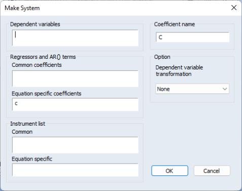
• provides an easy way to define a system without having to type in every equation. Dependent variables allows you to list the dependent variables in the system. You have the option to transform these variables by selecting from the Dependent variable transformation list in the Option section. Regressors and AR( ) terms that share the same coefficient across equations can be listed in Common coefficients, while those that do not can be placed in Equation specific coefficients. Command instruments can be listed in the Common field in the Instrument list section.
• opens the dialog for estimating the system of equations. It may also be accessed by pressing on the system toolbar.
• creates a number of series containing the residuals for each equation in the system. The residuals will be given the next unused name of the form RESID01, RESID02, etc., in the order that the equations are specified in the system.
• creates an untitled group object containing the endogenous variables.
• (for system ARCH) creates a series containing the log likelihood contribution.
• (for system ARCH) allows you to generate estimates of the conditional variances, covariances, or correlations for the specified set of dependent variables. (EViews automatically places all of the dependent variables in the Variable field. You have the option to modify this field to include only the variable of interest.)
If you select Group under Format, EViews will save the data in series. The Base name edit box indicates the base name to be used when generating series data. For the conditional variance series, the naming convention will be the specified base name plus terms of the form “_01”, “_02”. For covariances or correlations, the naming convention will use the base name plus “_01_02”, “_01_03”, etc., where the additional text indicates the covariance/correlation between member 1 and 2, member 1 and 3, etc.
If Matrix is selected then whatever is in the Matrix name field will be generated for what is in the Date (or Presample if it is checked) edit field.
Example
As an illustration of the process of estimating a system of equations in EViews, we estimate a translog cost function using data from Berndt and Wood (1975) as presented in Greene (1997). The data are provided in “G_cost.WF1”. The translog cost function has four factors with three equations of the form:
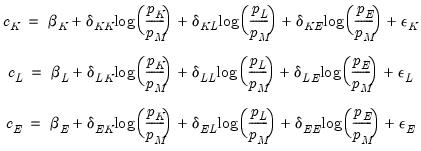 | (43.5) |
where

and

are the cost share and price of factor

, respectively.

and

are the parameters to be estimated. Note that there are cross equation coefficient restrictions that ensure symmetry of the cross partial derivatives.
We first estimate this system without imposing the cross equation restrictions and test whether the symmetry restrictions hold. Create a system by clicking in the main toolbar or type system in the command window. Press the button and type in the name “SYS_UR” to name the system.
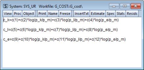
Next, type in the system window and specify the system as:
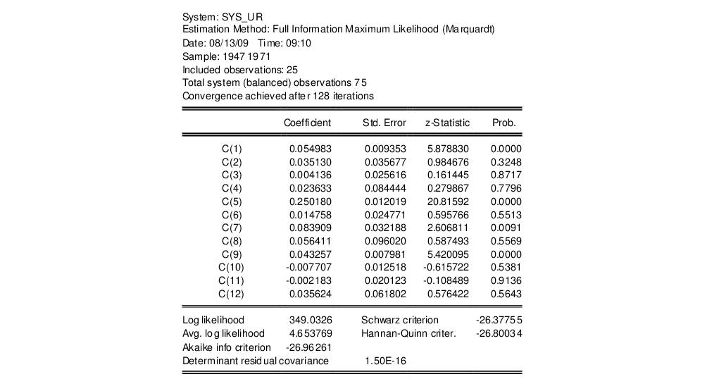
We estimate this model by full information maximum likelihood (FIML). FIML is invariant to the equation that is dropped. Press the button and choose Full Information Maximum Likelihood. Click on to perform the estimation. EViews presents the estimated coefficients and regression statistics for each equation. The top portion of the output describes the coefficient estimates:
while the bottom portion of the output (not depicted) describes equation specific statistics.
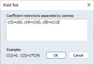
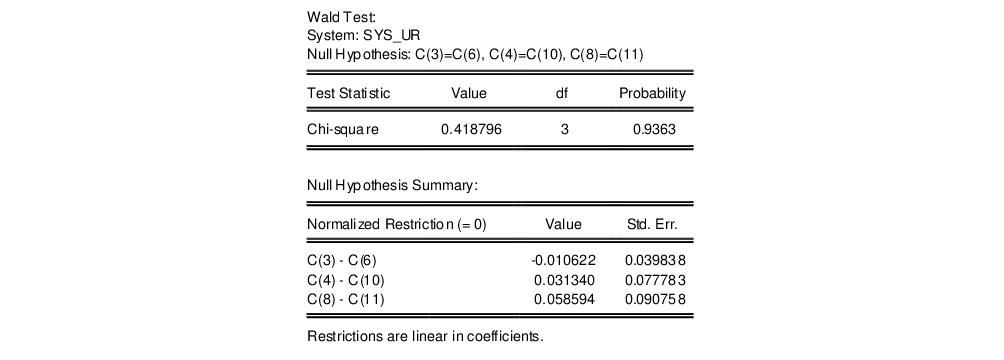
To test the symmetry restrictions, select , fill in the dialog:
and click . The test result:
fails to reject the symmetry restrictions. To estimate the system imposing the symmetry restrictions, copy the object using click and modify the system.
We have named the system SYS_TLOG. Note that to impose symmetry in the translog specification, we have restricted the coefficients on the cross-price terms to be the same (we have also renumbered the 9 remaining coefficients so that they are consecutive). The restrictions are imposed by using the same coefficients in each equation. For example, the coefficient on the log(P_L/P_M) term in the C_K equation, C(3), is the same as the coefficient on the log(P_K/P_M) term in the C_L equation.
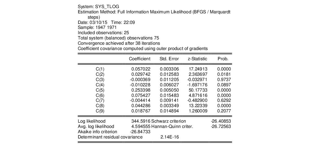
To estimate this model using FIML, click and choose Full Information Maximum Likelihood. We will leave the combo at the default setting of to allow for estimation of an unrestricted covariance matrix. Click on to estimate the equation.
The top part of the equation describes the estimation specification, and provides coefficient and standard error estimates, t-statistics, p-values, and summary statistics:
The log likelihood value reported at the bottom of the first part of the table may be used to construct likelihood ratio tests.
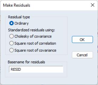
Since maximum likelihood assumes the errors are multivariate normal, we may wish to test whether the residuals are normally distributed. Click to display the residuals dialog. You may choose to save the ordinary or standardized residuals. If you choose the latter, you can elect to standardize the residuals using the Cholesky factor of the (conditional) covariance, the square root of the (conditional) correlation matrix, or the square root of the (conditional) covariance matrix. You must enter a basename for saving the residuals. The residuals will be named using the next available names in the workfile, in this case “RESID01”, “RESID02”, ...., if those names are not already used.
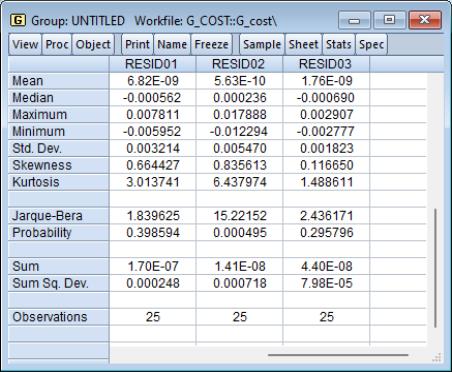
In this example, we elect to produce ordinary residuals. EViews opens an untitled group window containing the residuals of each equation in the system. To compute descriptive statistics for each residual in the group, select from the group window toolbar.
The Jarque-Bera statistic rejects the hypothesis of normal distribution for the second equation but not for the other equations.
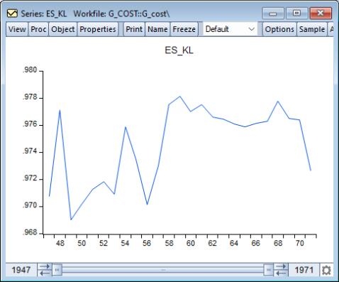
The estimated coefficients of the translog cost function may be used to construct estimates of the elasticity of substitution between factors of production. For example, the elasticity of substitution between capital and labor is given by 1+c(3)/(C_K*C_L). Note that the elasticity of substitution is not a constant, and depends on the values of C_K and C_L. To create a series containing the elasticities computed for each observation, select , and enter:
es_kl = 1 + sys_tlog.c(3)/(c_k*c_l)
To plot the series of elasticity of substitution between capital and labor for each observation, double click on the series name ES_KL in the workfile and select :
While it varies over the sample, the elasticity of substitution is generally close to one, which is consistent with the assumption of a Cobb-Douglas cost function.
System ARCH Example
In this section we provide an example for system arch estimation. We will model the weekly returns of Japanese Yen (

), Swiss Franc (

) and British Pound (

). The data, which are located in the WEEKLY page of the workfile “Fx.WF1”, which may be located in the Example File folder, contain the weekly exchange rates of these currencies against the U.S. dollar. The mean equations for the continuously compounding returns is regressed against a constant:
 | (43.6) |
where
is assumed to distributed normally with mean zero and covariance

. The conditional covariance is modeled with a basic Diagonal VECH model:
 | (43.7) |
To estimate this model, create a system SYS01 with the following specification:
dlog(jy) = c(1)
dlog(sf) = c(2)
dlog(bp) = c(3)
We estimate this model by selecting ARCH - Conditional Heteroskedasticity as the estimation method in the estimation dialog. Since the model we want to estimate is the default Diagonal VECH model we leave most of the settings as they are. In the sample field, we change the sample to “1980 2000” to use only a portion of the data. Click on OK to estimate the system.
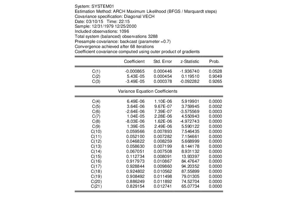
EViews displays the results of the estimation, which are similar to other system estimation output with a few differences. The ARCH results contain the coefficients statistics section (which includes both the mean and raw variance coefficients), model and equation specific statistics, and an extended section describing the variance coefficients.
The coefficient section at the top is separated into two parts, one contains the estimated coefficient for the mean equation and the other contains the estimated raw coefficients for the variance equation. The parameters estimates of the mean equation, C(1), C(2) and C(3), are listed in the upper portion of the coefficient list.
The variance coefficients are displayed in their own section. Coefficients C(4) to C(9) are the coefficients for the constant matrix, C(10) to C(15) are the coefficients for the ARCH term, and C(16) through C(21) are the coefficients for the GARCH term.
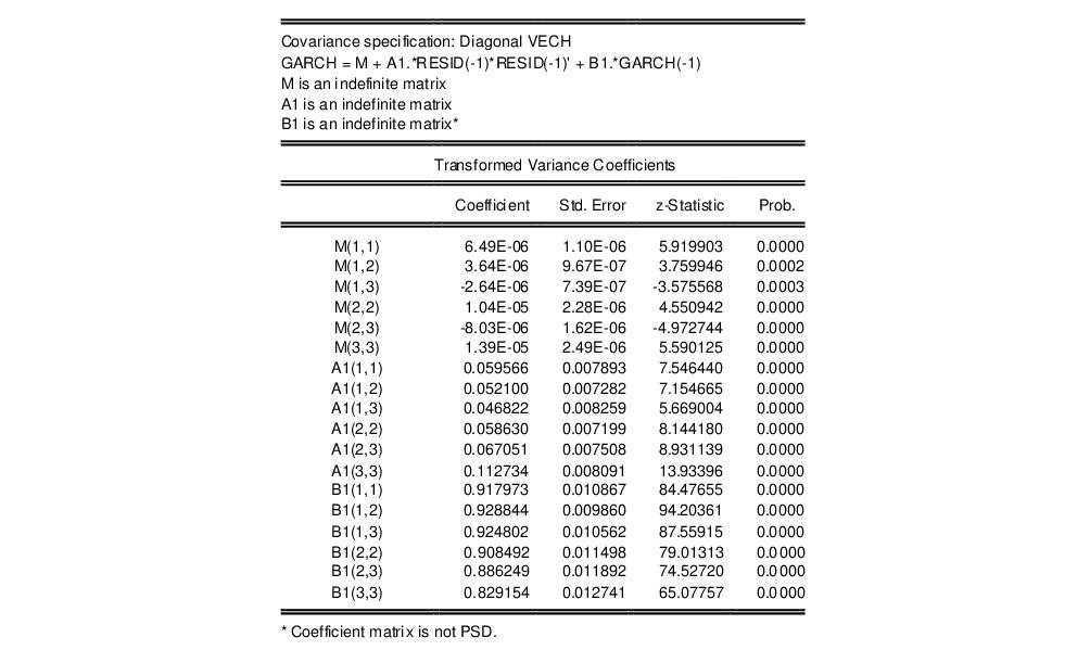
Note that the number of variance coefficients in an ARCH model can be very large. Even in this small 3-variable system, 18 parameters are estimated, making interpretation somewhat difficult. To aid you in interpreting the results, EViews provides a covariance specification section at the bottom of the estimation output that re-labels and transforms coefficients:
The first line of this section states the covariance model used in estimation, in this case Diagonal VECH. The next line of the header describes the model that we have estimated in abbreviated text form. In this case, “GARCH” is the conditional variance matrix, “M” is the constant matrix coefficient, A1 is the coefficient matrix for the ARCH term and B1 is the coefficient matrix for the GARCH term. M, A1, and B1 are all specified as indefinite matrices.
Next, the estimated values of the matrix elements as well as other statistics are displayed. Since the variance matrices are indefinite, the values are identical to those reported for the raw variance coefficients. For example, M(1,1), the (1,1) element in matrix M, corresponds to raw coefficient C(4), M(1,2) corresponds to C(5), A1(1,1) to C(10), etc.
For matrix coefficients that are rank 1 or full rank, the values reported in this section are a transformation of the raw estimated coefficients, i.e. they are a function of one or more of the raw coefficients. Thus, the reported values do not have a one-to-one correspondence with the raw parameters.
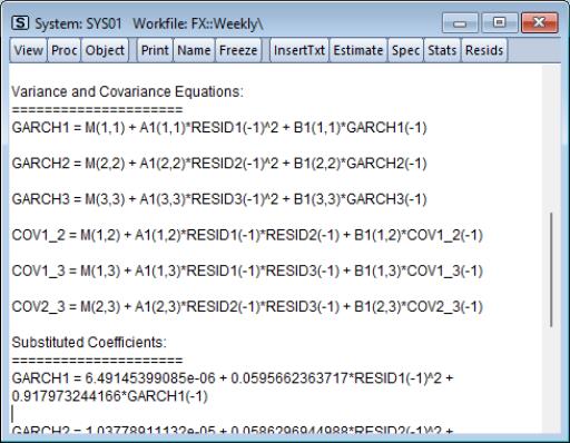
A single equation representation of the variance-covariance equation may be viewed by clicking on and scrolling down to the Variance and Covariance Equations section.
The GARCH equations are the conditional variance equations while the COV equations are the conditional covariance equations. For example GARCH1 is the conditional variance of Japanese yen. COV1_2 is the conditional covariance between the Japanese Yen and the Swiss Franc.
Before proceeding we name the system SYS01 by clicking on the button and accepting the default name.
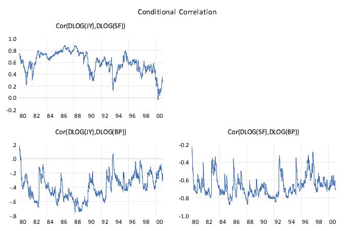
A graph of the conditional variance can be generated using . An extensive list of options is available, including Covariance, Correlation, Variance, and Standard Deviation. Data may also be displayed in graph, matrix or time series list format. Here is the correlation view:
The correlation looks to be time varying, which is a general characteristic of this model.
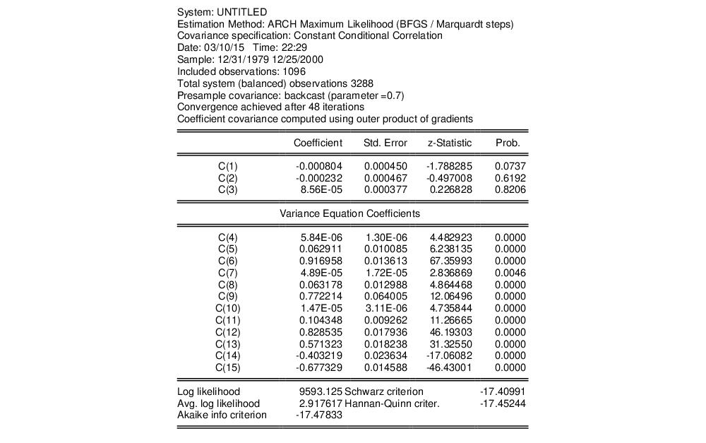
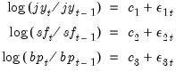
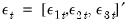
Another possibility is to model the covariance matrix using the CCC specification, which imposes a constant correlation over time. We proceed by creating a new system with specification identical to the one above. We'll select Constant Conditional Correlation this time as the for estimation and leave the remaining settings as they are. The basic results:
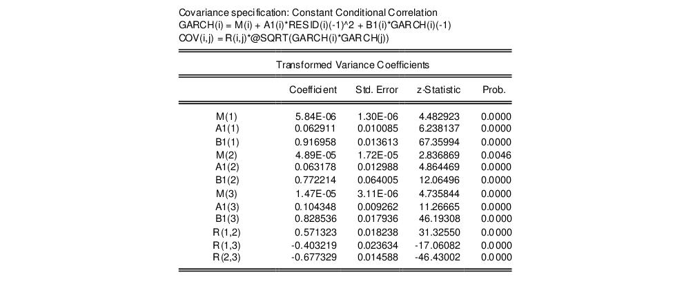
Note that this specification has only 12 free parameters in the variance equation, as compared with 18 in the previous model. The extended variance section represents the variance equation as,
GARCH(i) = M(i) + A1(i)*RESID(i)(-1)^2 + B1(i)*GARCH(i)(-1)
while the model for the covariance equation is:
COV(i,j) = R(i,j)*@SQRT(GARCH(i)*GARCH(j))
The lower portion of the output shows that the correlations, R(1, 2), R(1, 3), and R(2, 3) are 0.5713, -0.4032, and -0.6773, respectively:
Is this model better than the previous model? While the log likelihood value is lower, it also has fewer coefficients. We may compare the two system by looking at model selection criteria. The Akaike, Schwarz and Hannan-Quinn all show lower information criteria values for the VECH model than the CCC specification, suggesting that the time-varying Diagonal VECH specification may be preferred.