Views and Procs of a VAR
Once you have estimated a VAR, EViews provides various views and procs to work with the estimated VAR.
In this section, we discuss views that are specific to VARs. For other views and procedures, see the general discussion of system views in
“System Estimation”.
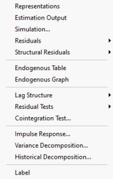
Residual Views
You may use the entries under the and menus to examine the residuals of the estimated VAR in graph or spreadsheet form, or you may examine the covariance and correlation matrix of those residuals.
The views listed under will display results using the raw residuals from the estimated VAR.
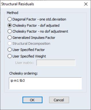
Alternately, you may display the views to examine the these transformed estimated residuals. If the

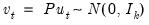
are the ordinary residuals, we may plot the structural residuals

based on factor loadings

,
 | (44.23) |
or based on weights

,
 | (44.24) |
When producing results for the views, you will be prompted to choose a transformation.
Note that there is a corresponding procs which will save the residuals series in the workfile ( and ).
Diagnostic Views
A set of diagnostic views are provided under the menus and in the VAR window. These views should help you check the appropriateness of the estimated VAR.
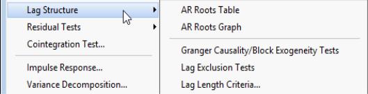
Lag Structure
EViews offers several views for investigating the lag structure of your equation.
AR Roots Table/Graph
Reports the
inverse roots of the characteristic AR polynomial; see Lütkepohl (1991). The estimated VAR is stable (stationary) if all roots have modulus less than one and lie inside the unit circle. If the VAR is not stable, certain results (such as impulse response standard errors) are not valid. There will be

roots, where

is the number of endogenous variables and

is the largest lag. If you estimated a VEC with

cointegrating relations,

roots should be equal to unity.
Pairwise Granger Causality Tests
Carries out pairwise Granger causality tests and tests whether an endogenous variable can be treated as exogenous. For each equation in the VAR, the output displays

(Wald) statistics for the joint significance of each of the other lagged endogenous variables in that equation. The statistic in the last row (
All) is the

-statistic for joint significance of all other lagged endogenous variables in the equation.
Warning: if you have estimated a VEC, the lagged variables that are tested for exclusion are only those that are first differenced. The lagged level terms in the cointegrating equations (the error correction terms) are not tested.
Note: for VAR models with linear restrictions, EViews will only perform tests involving endogenous variable lags for which there are no restrictions.
Lag Exclusion Tests
Carries out lag exclusion tests for each lag in the VAR. For each lag, the

(Wald) statistic for the joint significance of all endogenous variables at that lag is reported for each equation separately and jointly (last column).
Note: for VAR models with linear restrictions, EViews will only perform tests involving endogenous variable lags for which there are no restrictions.
Lag Length Criteria
Computes various criteria to select the lag order of an unrestricted VAR. You will be prompted to specify the maximum lag to “test” for. The table displays various information criteria for all lags up to the specified maximum. (If there are no exogenous variables in the VAR, the lag starts at 1; otherwise the lag starts at 0.) The table indicates the selected lag from each column criterion by an asterisk “*”. For columns 4–7, these are the lags with the smallest value of the criterion.
All the criteria are discussed in Lütkepohl (1991, Section 4.3). The sequential modified likelihood ratio (LR) test is carried out as follows. Starting from the maximum lag, test the hypothesis that the coefficients on lag

are jointly zero using the

statistics:
 | (44.25) |
where

is the number of parameters per equation under the alternative. Note that we employ Sims’ (1980) small sample modification which uses (

) rather than

. We compare the modified LR statistics to the 5% critical values starting from the maximum lag, and decreasing the lag one at a time until we first get a rejection. The alternative lag order from the first rejected test is marked with an asterisk (if no test rejects, the minimum lag will be marked with an asterisk). It is worth emphasizing that even though the individual tests have size 0.05, the overall size of the test will not be 5%; see the discussion in Lütkepohl (1991, p. 125–126).
Note: for VAR models with linear restrictions, EViews perform lag length tests using models in which the VAR linear restrictions are not applied.
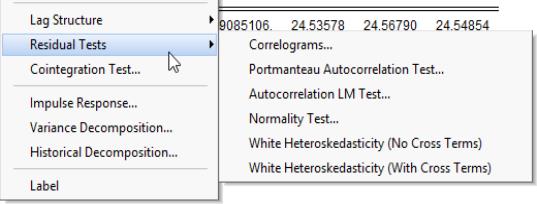
Residual Tests
You may use these views to examine the properties of the residuals from your estimated VAR.
Correlograms
Displays the pairwise cross-correlograms (sample autocorrelations) for the estimated residuals in the VAR for the specified number of lags. The cross-correlograms can be displayed in three different formats. There are two tabular forms, one ordered by variables (
Tabulate by Variable) and one ordered by lags (
Tabulate by Lag). The
Graph form displays a matrix of pairwise cross-correlograms. The dotted line in the graphs represent plus or minus two times the approximate asymptotic standard errors of the lagged correlations (ignoring coefficient estimation and computed as

).
Portmanteau Autocorrelation Test
Computes the multivariate Box-Pierce/Ljung-Box
Q-statistics for residual serial correlation up to the specified order (see Lütkepohl, 1991, 4.4.21 & 4.4.23 for details). We report both the
Q-statistics and the adjusted
Q-statistics (with a small sample correction). Under the null hypothesis of no serial correlation up to lag

, both statistics are
approximately distributed

with degrees of freedom

where

is the VAR lag order if there are no coefficient restrictions, and

where

contains adjustments for the restrictions.
The asymptotic distribution is approximate in the sense that it requires the MA coefficients to be zero for lags

. Therefore, this approximation will be poor if the roots of the AR polynomial are close to one and

is small. In fact, the degrees of freedom becomes negative for

.
Note that adjustments are made to the computation of the p-value of these statistics when the model is a VECM (Brüggemann, Lütkepohl, and Saikkonen, 2006).
Autocorrelation LM Test
Reports the multivariate LM test statistics for residual serial correlation up to the specified order. A Breusch-Godfrey test statistic for autocorrelation at lag order

is computed by running an auxiliary regression of the residuals

on the original right-hand regressors and the lagged residual

, where the missing first

values of

are filled with zeros.
See Johansen (1995, p. 22) for the formula of the LR version of this LM test. The form of this statistic employs the Edgeworth expansion correction (Edgerton and Shukur 1999). Under the null hypothesis of no serial correlation of order

, the LM statistic is asymptotically distributed

with

degrees of freedom.
A variant of this test tests for autocorrelation for lags 1 to

. The test modifies the LM statistic above by including all of the modified lagged residual regressors from

. Under the null hypothesis, the LM statistic is asymptotically

with

degrees of freedom.
In addition to the LR version of the test, EViews computes the Rao F-test version of the LM statistic as described Edgerton and Shukur (1999) since their simulations suggest it performs best among the many variants they consider.
Normality Test
This view reports the multivariate extensions of the Jarque-Bera residual normality test, which compares the third and fourth moments of the residuals to those from the normal distribution. For the multivariate test, you must choose a factorization of the

residuals that are orthogonal to each other (see
“Impulse Responses” for additional discussion of the need for orthogonalization).
Let

be a

factorization matrix such that:
 | (44.26) |
where

is the demeaned residuals. Define the third and fourth moment vectors
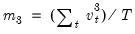
and
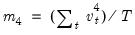
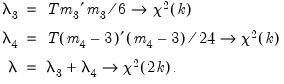
. Then:
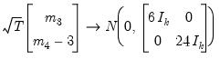 | (44.27) |
under the null hypothesis of normal distribution. Since each component is independent of each other, we can form a

-statistic by summing squares of any of these third and fourth moments.
EViews provides you with choices for the factorization matrix

:
• Cholesky (Lütkepohl 1991, p. 155-158):

is the inverse of the lower triangular Cholesky factor of the residual covariance matrix. The resulting test statistics depend on the ordering of the variables in the VAR.
• Inverse Square Root of Residual Correlation Matrix (Doornik and Hansen 1994):
where

is a diagonal matrix containing the eigenvalues of the residual correlation matrix on the diagonal,

is a matrix whose columns are the corresponding eigenvectors, and

is a diagonal matrix containing the inverse square root of the residual variances on the diagonal. This

is essentially the inverse square root of the residual correlation matrix. The test is invariant to the ordering and to the scale of the variables in the VAR. As suggested by Doornik and Hansen (1994), we perform a small sample correction to the transformed residuals

before computing the statistics.
• Inverse Square Root of Residual Covariance Matrix (Urzua 1997):
where

is the diagonal matrix containing the eigenvalues of the residual covariance matrix on the diagonal and

is a matrix whose columns are the corresponding eigenvectors. This test has a specific alternative, which is the quartic exponential distribution. According to Urzua, this is the “most likely” alternative to the multivariate normal with finite fourth moments since it can approximate the multivariate Pearson family “as close as needed.” As recommended by Urzua, we make a small sample correction to the transformed residuals

before computing the statistics. This small sample correction differs from the one used by Doornik and Hansen (1994); see Urzua (1997, Section D).
• Factorization from Identified (Structural) VAR:

where

,

are estimated from the structural VAR model. This option is available only if you have estimated the factorization matrices

and

using the structural VAR (see
(here)).
EViews reports test statistics for each orthogonal component (labeled RESID1, RESID2, and so on) and for the joint test. For individual components, the estimated skewness

and kurtosis

are reported in the first two columns together with the
p-values from the

distribution (in square brackets). The Jarque-Bera column reports:
 | (44.28) |
with
p-values from the

distribution.
Note: in contrast to the Jarque-Bera statistic computed in the series view, this statistic is not computed using a degrees of freedom correction.For the joint tests, we will generally report:
 | (44.29) |
If, however, you choose Urzua’s (1997) test,

will not only use the sum of squares of the “pure” third and fourth moments but will also include the sum of squares of all
cross third and fourth moments. In this case,

is asymptotically distributed as a

with
degrees of freedom.
White Heteroskedasticity Test
These tests are the extension of White’s (1980) test to systems of equations as discussed by Kelejian (1982) and Doornik (1995). The test regression is run by regressing each cross product of the residuals on the cross products of the regressors and testing the joint significance of the regression. The No Cross Terms option uses only the levels and squares of the original regressors, while the With Cross Terms option includes all non-redundant cross-products of the original regressors in the test equation. The test regression always includes a constant term as a regressor.
The first part of the output displays the joint significance of the regressors excluding the constant term for each test regression. You may think of each test regression as testing the constancy of each element in the residual covariance matrix separately. Under the null of no heteroskedasticity or (no misspecification), the non-constant regressors should not be jointly significant.
The last line of the output table shows the LM chi-square statistics for the joint significance of all regressors in the system of test equations (see Doornik, 1995, for details). The system LM statistic is distributed as a

with degrees-of-freedom

, where
is the number of cross-products of the residuals in the system and

is the number of the common set of right-hand side variables in the test regression.
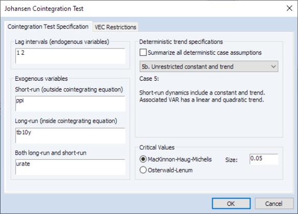
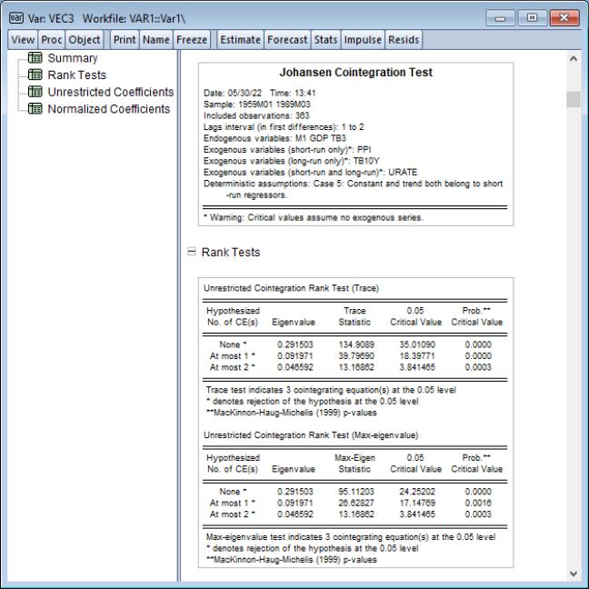
Cointegration Test
This view performs the Johansen cointegration test for the variables in your VAR. Note that Johansen cointegration tests may also be performed from a Group object.
To perform the test, select from an estimated VAR object window using. In the latter case, the test dialog will be pre-filled with information from the VAR (or VEC) specification:
Enter the lag specification and exogenous variables specifications in the appropriate edit fields, and specify the deterministic trend specifications using the dropdown. The checkbox may be used to compute the test statistic for all of the deterministic trend cases.
See
“Johansen Cointegration Test” for a description of the basic test methodology and test settings. See also
“The VECM Specification” and
“Estimating VEC Models in EViews” for a discussion of VEC specifications.
Bear in mind that the lag specification for is for the error correction form of the VEC model, not the levels of a VAR. If performing the test on a specification in levels as in an ordinary VAR, the lag structure will differ in the test equation.
Similarly, note that exogenous variables in a VAR will be placed in the edit field, which may not be the desired test specification in the error correction form of the VEC.
Notes on System Comparability
Many of the diagnostic tests given above may be computed “manually” by estimating the VAR using a system object and selecting We caution you that the results from the system may not match those from the VAR diagnostic views for various reasons:
• The system object will, in general, use the maximum possible observations for each equation in the system. By contrast, VAR objects force a balanced sample across equations in cases where there are missing values.
• The estimates of the weighting matrix used in system estimation do not contain a degrees of freedom correction (the residual sums-of-squares are divided by

rather than by

), while the VAR estimates do perform this adjustment. Even though estimated using comparable specifications and yielding identifiable coefficients, the test statistics from system SUR and the VARs will show small (asymptotically insignificant) differences.
Impulse Responses
Interpreting VAR results can be difficult due to the complex interdependence between variables, their lags, and the large number of coefficients in the model. Notably, a shock to the i-th variable not only directly affects the i-th variable but is also transmitted to all of the other endogenous variables through the dynamic (lag) structure of the VAR.
A primary method of examining the properties of a VAR or VEC is impulse response (IR) analysis, which traces the impact of a shock to a single variable on the current and future values of all of the endogenous variables.
EViews offers a wide range of options for computing impulse-responses, estimating the precision of those estimates, and displaying the results.
“Impulse Response Analysis” offers background and a description of these tools.
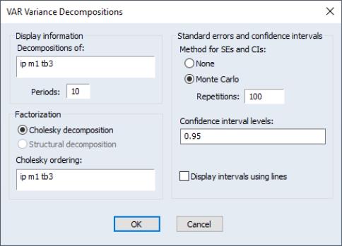
Variance Decomposition
While impulse response functions trace the effects of a shock to one endogenous variable on to the other variables in the VAR, variance decomposition separates the variation in an endogenous variable into the component shocks to the VAR. Thus, the variance decomposition provides information about the relative importance of each random innovation in affecting the variables in the VAR.
To obtain the variance decomposition, select from the VAR object toolbar. You should provide the same information as for impulse responses above.
Note that since non-orthogonal factorization will yield decompositions that do not satisfy an adding up property, your choice of factorization is limited to the and the , the latter if available.
The table format displays a separate variance decomposition for each endogenous variable. The second column, labeled “S.E.”, contains the forecast error of the variable at the given forecast horizon. The source of this forecast error is the variation in the current and future values of the innovations to each endogenous variable in the VAR. The remaining columns give the percentage of the forecast variance due to each innovation, with each row adding up to 100.
As with the impulse responses, the variance decomposition based on the Cholesky factor can change dramatically if you alter the ordering of the variables in the VAR. For example, the first period decomposition for the first variable in the VAR ordering is completely due to its own innovation.
Factorization based on structural orthogonalization is available only if you have estimated the structural factorization matrices as explained in
“Structural (Identified) VARs”. Note that the forecast standard errors should be identical to those from the Cholesky factorization
if the structural VAR is just identified. For over-identified structural VARs, the forecast standard errors may differ in order to maintain the adding up property.
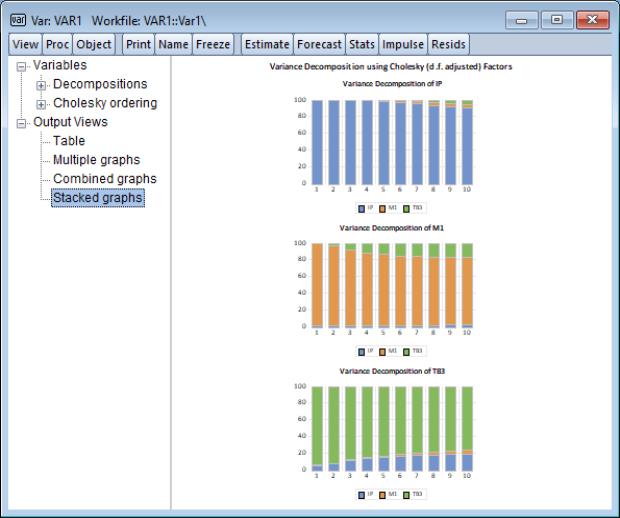
As with the output for impulse responses (
“Impulse Responses”), the resulting output is interactive. You may click on any of the node entries to change the display type. Here we see a representation of the decomposition.
Similarly, you may click on the node under and toggle on the variable names to show or hide the display of the decomposition of specific variables.
Historical Decomposition
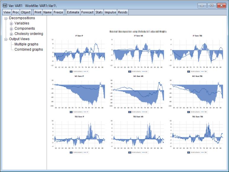
An alternative method of innovation accounting is to decompose the observed series into the components corresponding to each structural shock. Burbridge and Harrison (1985) propose transforming observed residuals to structural residuals, and then for each observation beyond some point in the estimation sample, computing the contribution of the different accumulated structural shocks to each observed variable.
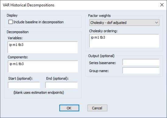
To obtain the historical decomposition, select from the VAR object toolbar. You should provide the same information as for impulse responses and variance decomposition above.
In addition, you may use the to choose whether to include the base projection in the decomposition, or whether to plot only the stochastic accumulations and total.
Lastly, you may use the edit fields to specify an optional and period to the decomposition. Both periods must be within the range of the original estimation period. If you leave the fields blank, EViews will perform the decomposition from the start to the end of the full estimation period.
Procs of a VAR
Most of the procedures available for a VAR are common to those available for a system object (see
“System Procs”). Here, we discuss only those procedures that are unique to the VAR object.
Forecasting
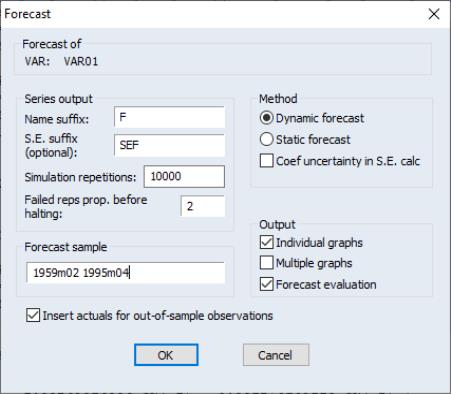
You may produce forecasts directly from an estimated VAR object by clicking on the button or by selecting . EViews will display the forecast dialog:
Most of the dialog should be familiar from the standard equation forecast dialog. There are, however, a few minor differences.
First, the fields in which you enter the forecast name and optional S.E. series names now refer to the character suffix which you will use to form output series names. By default, as depicted here, EViews will append the letter “f” to the end of the original series names to form the output series names. If necessary, the original name will be converted into a valid EViews series name.
Second, if you choose to compute standard errors of the forecast, EViews will obtain those values via simulation. You will be prompted for the number of , and the “” the simulation setting.
Lastly, in addition to a , you are given a choice of whether to display the output graphs as , as , or both.
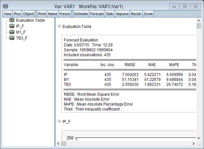
Clicking on instructs EViews to perform the forecast and, if appropriate to display the output:
In this case, the output consists of a spool containing the forecast evaluation of the series in the VAR, along with individual graphs of the forecasts and the corresponding actuals series.
Make System
This proc creates a system object that contains an equivalent VAR specification. If you want to estimate a non-standard VAR, you may use this proc as a quick way to specify a VAR in a system object which you can then modify to meet your needs. For example, while the VAR object requires each equation to have the same lag structure, you may want to relax this restriction. To estimate a VAR with unbalanced lag structure, use the procedure to create a VAR system with a balanced lag structure and edit the system specification to meet the desired lag specification.
The option creates a system whose specification (and coefficient number) is ordered by variables. Use this option if you want to edit the specification to exclude lags of a specific variable from some of the equations. The option creates a system whose specification (and coefficient number) is ordered by lags. Use this option if you want to edit the specification to exclude certain lags from some of the equations.
For vector error correction (VEC) models, treating the coefficients of the cointegrating vector as additional unknown coefficients will make the resulting system unidentified. In this case, EViews will create a system object where the coefficients for the cointegrating vectors are fixed at the estimated values from the VEC. If you want to estimate the coefficients of the cointegrating vector in the system, you may edit the specification, but you should make certain that the resulting system is identified.
You should also note that while the standard VAR can be estimated efficiently by equation-by-equation OLS, this is generally not the case for the modified specification. You may wish to use one of the system-wide estimation methods (e.g., SUR) when estimating non-standard VARs using the system object.
Estimate Structural Factorization
This procedure is used to estimate the factorization matrices for a structural (or identified) VAR. The details for this procedure are provided in
“Structural (Identified) VARs” below. You must first estimate the structural factorization matrices using this proc in order to use the structural options in impulse responses and variance decompositions.