Graph
Graph object. Specialized object used to hold graphical output.
Graph Declaration
freeze freeze graphical view of object.
graph create graph object using graph command or by merging existing graphs.
Graphs may be created by declaring a graph using one of the graph commands described below, or by freezing the graphical view of an object. For example:
graph myline.line ser1
graph myscat.scat ser1 ser2
graph myxy.xyline grp1
declare and create the graph objects MYLINE, MYSCAT and MYXY. Alternatively, you can use the freeze command to create graph objects:
freeze(myline) ser1.line
group grp2 ser1 ser2
freeze(myscat) grp2.scat
freeze(myxy) grp1.xyline
which are equivalent to the declarations above.
Graph Type Commands
Graph creation types are discussed in detail in
“Graph Creation Command Summary”.
bubbletrip bubble plot graph specified as triplets.
hilo high-low(-open-close) graph.
qqplot quantile-quantile graph.
Graph View
display display table, graph, or spool in object window.
label label information for the graph.
Graph Procs
addarrow draw a line or arrow on a graph.
addrect draw a rectangle on a graph.
addtext place arbitrary text on the graph.
align align the placement of multiple graphs.
axis set the axis scaling and display characteristics for the graph.
clearhist clear the contents of the history attribute.
copy creates a copy of the graph.
datalabel controls labeling of the observations/data in time plots. (
new)
datelabel controls labeling of the bottom date/time axis in time plots.
delete removes all objects of specified type from a graph object.
draw draw lines and shaded areas on the graph.
drawdefault set default settings for lines and shaded areas on the graph.
legend control the appearance and placement of legends.
makegroup creates a group object containing all the series in the graph.
merge merge graph objects.
name change the series name for legends or axis labels.
olepush push updates to OLE linked objects in open applications.
options change the option settings of the graph.
save save graph to a graphics file.
setattr set the value of an object attribute.
setbpelem set options for element of a boxplot graph.
setelem set individual line, symbol, bar and legend options for each series in the graph.
setfont set the font for the text in a graph.
setobslabel set custom axis labels for observation scale of a graph.
sort sort the series in a graph.
textdefault set default settings for text objects in the graph.
update update graph with data changes.
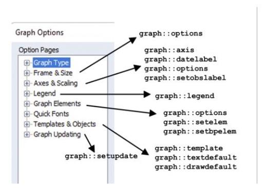
The relationship between the elements of the graph dialog and the associated graph procs is illustrated below:
Graph Data Members
Scalar Values
@axismin(axis) returns the minimum value for the specified axis. Acceptable values for axis are “t”, “l”, “b”, “r”, for top, left, bottom, right.
@axismax(axis) returns the maximum value for the specified axis. Acceptable values for axis are “t”, “l”, “b”, “r”, for top, left, bottom, right.
@axispos(value, axis) returns the location in virtual inches of the specified data value on the graph. value is in the same units as the specified axis. When specifying a date for value, the string must be quoted. Acceptable values for axis are “t”, “l”, “b”, “r” for top, left, bottom, right.
String Values
@attr("arg") string containing the value of the arg attribute, where the argument is specified as a quoted string.
@description returns a string containing the object description (if available).
@detailedtype returns a string with the object type: “GRAPH”.
@displayname returns a string containing the Graph’s displayname. If the Graph has no display name set, the name is returned.
@members string containing a space delimited list of the names of the series contained in the Graph.
@name returns a string containing the Graph’s name.
@remarks returns a string containing the Graph’s remarks (if available).
@type returns a string with the object type: “GRAPH”.
@updatetime returns a string representation of the time and date at which the Graph was last updated.
Graph Examples
You can declare your graph:
graph abc.xyline(m) unemp gnp inf
graph bargraph.bar(d,l) unemp gnp
Alternately, you may freeze any graphical view:
freeze(mykernel) ser1.distplot kernel
You can change the graph type,
graph mygraph.line ser1
mygraph.hist
or combine multiple graphs:
graph xyz.merge graph1 graph2
Draw a line or arrow on a graph.
Syntax
graph_name.addarrow [pos(x1,y1,x2,y2) axispos(x1,y1,x2,y2,x-axis,y-axis) axispos(x1,y1,x2,y2,y-axis) axispt(x2,y2,angle,length,x-axis,y-axis)] linewidth(lwidth) arrowwidth(awidth) color(color) pattern(pattern) startsym(ssym) endsym(esym) label(str) labelpos(position) frame(size) indicator
Follow the addarrow keyword a set of specifications determining the position and style of the line/arrow to be drawn.
The position and size of the arrow/line can be specified with one of the pos, axispos or axispt arguments.
The
pos argument specifies coordinates of the line in virtual space.
x1 is the starting X (horizontal) coordinate, and
y1 is the starting Y (vertical) coordinate. Similarly
x2 and
y2 are the end point coordinates. Coordinates are set in virtual inches. Individual graphs are always

virtual inches (scatter diagrams are

virtual inches) or a user-specified size, regardless of their current display size.
The origin of the coordinate is the upper left hand corner of the graph. The x1 number specifies how many virtual inches to offset to the right from the origin. The second number y1 specifies how many virtual inches to offset below the origin. The start point of the line will be set at the specified coordinates.
The axispos argument specifies coordinates in units of the graph scale. x1 is the starting X (horizontal) coordinate, and y1 is the starting Y (vertical) coordinate. Similarly x2 and y2 are the end point coordinates.
For time-series graphs you must also specify which non-time based axis the y-coordinates’s scale are based on, using l,t,r,b for left, top, right, bottom respectively. x-coordinates should be specified as a date/time.
For non-time series graphs you must specify the axis of scale of both x and y coordinates.
The axispt argument specifies the end point coordinates of the line, along with the angle and length of the line. Angles are measured in degrees, and length in virtual inches.
The linewidth argument specifies the thickness of the line. lwidth should be a number between “.25” and “5”, indicating the width in points.
Arrowwidth determines the size of the arrow head on the line. awidth can be either “small”, “medium” or “large”.
color specifies the color of the line. The color value may set by using one of the color keywords (e.g., “blue”), by using the RGB values (e.g., “@RGB(255, 255, 0)”), or by specifying the components in hexadecimal (e.g., “@HEX(ff0000)”).
The predefined colors are given by the keywords (with their RGB and HEX equivalents):
blue | @rgb(0, 0, 255) | @hex(0000ff) |
red | @rgb(255, 0, 0) | @hex(ff0000) |
ltred | @rgb(255, 168, 168) | @hex(ffa8a8) |
green | @rgb(0, 128, 0) | @hex(008000) |
black | @rgb(0, 0, 0) | @hex(000000) |
white | @rgb(255, 255, 255) | @hex(ffffff) |
purple | @rgb(128, 0, 128) | @hex(800080) |
orange | @rgb(255, 128, 0) | @hex(ff8000) |
yellow | @rgb(255, 255, 0) | @hex(ffff00) |
gray | @rgb(128, 128, 128) | @hex(808080) |
ltgray | @rgb(192, 192, 192) | @hex(c0c0c0) |
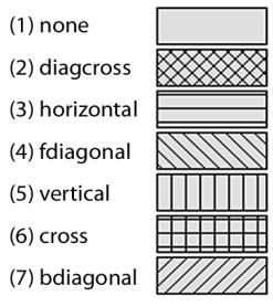
The pattern argument specifies the line pattern. pattern can take a numerical value, or one of the corresponding keywords:
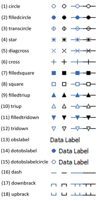
The startsym and endsym arguments define the arrowhead at the start or end of the line. You may specify “none”, “filled”, “outline”, or “rangeline”.
label adds a text label to the start point of the arrow. labelpos specifies the location of the text relative to the start point of the line. The following positions are available:
Vert | left or right of the start point depending on the angle of the line |
Horz | left or right of the start point depending on the angle of the line |
AR | above and right of the start point |
AL | above and left of the start point |
BR | below and right of the start point |
BL | below and left of the start point |
L | left of the start point |
R | right of the start point |
A | above the start point |
B | below the start point |
Frame encloses the text in a box. Size specifies whether the box should be a small box (sb) or a large box (lb).
Indicator places a red indicator within the text frame, indicating the start point location relative to the text. NOTE: The indicator will only appear if the label position (labelpos) is set to AR, AL, BR, or BL
Examples
The commands
create m 1990 2000
smpl 1990 1995
series y=nrnd
smpl 1995 2000
y = 6+nrnd
smpl @all
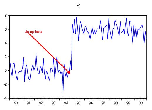
freeze(gr) y.line
gr.addarrow pos(0.7,0.65, 2.2,2.1) color(red) arrowwidth(large) endsym(outline) linewidth(2) label(Jump here)
create a graph and draw an arrow at the specified positions:
The command
gr.addarrow axispos(94, 3, 97, 4.2, l)
adds a second arrow starting at the point corresponding to the year 1994 on the x-axis and the y-axis value of 3, and ending at the year 1997 with a y-value of 4.2.
Cross-references
Draw an ellipse on a graph.
Syntax
graph_name.addellipse [pos(x1,y1,x2,y2) axisctr(x1,y1,x-axis,y-axis) axispos(x1,y1,y-axis)] linewidth(lwidth) color(color) pattern(pattern) height(height) width(width) angle(angle)
Follow the addellipse keyword a set of specifications determining the position and style of the ellipse to be drawn.
The position and size of the ellipse can be specified with either the pos or axisctr arguments.
The
pos argument specifies coordinates of the center of the ellipse in virtual space.
x1 is the center point X (horizontal) coordinate, and
y1 is the center point Y (vertical) coordinate. Coordinates are set in virtual inches. Individual graphs are always

virtual inches (scatter diagrams are

virtual inches) or a user-specified size, regardless of their current display size.
The origin of the coordinate is the upper left hand corner of the graph. The x1 number specifies how many virtual inches to offset to the right from the origin. The second number y1 specifies how many virtual inches to offset below the origin.
The axisctr argument specifies coordinates in units of the graph scale. x1 is the center point X (horizontal) coordinate, and y1 is the center point Y (vertical) coordinate.
For time-series graphs you must also specify which non-time based axis the y-coordinates’s scale are based on, using l,t,r,b for left, top, right, bottom respectively. x-coordinates should be specified as a date/time.
For non-time series graphs you must specify the axis of scale of both x and y coordinates.
The height argument specifies the height of the ellipse. Similarly the width argument specifies its width. angle controls the rotation of the ellipse (in degrees).
The linewidth argument specifies the thickness of the ellipse outline. lwidth should be a number between “.25” and “5”, indicating the width in points.
color specifies the color of the ellipse outline. The color value may set by using one of the color keywords (e.g., “blue”), by using the RGB values (e.g., “@RGB(255, 255, 0)”), or by specifying the components in hexadecimal (e.g., “@HEX(ff0000)”).
The predefined colors are given by the keywords (with their RGB and HEX equivalents):
blue | @rgb(0, 0, 255) | @hex(0000ff) |
red | @rgb(255, 0, 0) | @hex(ff0000) |
ltred | @rgb(255, 168, 168) | @hex(ffa8a8) |
green | @rgb(0, 128, 0) | @hex(008000) |
black | @rgb(0, 0, 0) | @hex(000000) |
white | @rgb(255, 255, 255) | @hex(ffffff) |
purple | @rgb(128, 0, 128) | @hex(800080) |
orange | @rgb(255, 128, 0) | @hex(ff8000) |
yellow | @rgb(255, 255, 0) | @hex(ffff00) |
gray | @rgb(128, 128, 128) | @hex(808080) |
ltgray | @rgb(192, 192, 192) | @hex(c0c0c0) |
The pattern argument specifies the ellipse outline pattern. pattern can take a numerical value, or one of the corresponding keywords:
Examples
The commands
create m 1990 2000
smpl 1990 1995
series y=nrnd
smpl 1995 2000
y = 6+nrnd
smpl @all
freeze(gr) y.line
gr.addellipse pos(1,1) width(2) height(.7) angle(110) color(red) pattern(2) linewidth(3)
create a graph and adds a red ellipse that is centered 1 virtual inch from the top and 1 virtual inch from the left of the graph that is 2 virtual inches wide and 0.7 virtual inches tall. It uses a 3 pt dash1 line pattern. The ellipse is also rotated 110 degrees
The command
gr.addellipse axisctr(1995, @mean(x),l) width(30) height(.2) angle(-50) color(blue)
adds to a blue ellipse that is centered at 1995 and the mean of x in left axis units. It is 30 observations wide and 0.2 left axis units tall. It is also rotated -50 degrees
Cross-references
Draw a rectangle on a graph.
Syntax
graph_name.addrect[pos(x1,y1,x2,y2) axisctr(x1,y1,x-axis,y-axis) axispos(x1,y1,y-axis)] linewidth(lwidth) color(color) pattern(pattern) height(height) width(width) angle(angle)
Follow the addrect keyword a set of specifications determining the position and style of the rectangle to be drawn.
The position and size of the rectangle can be specified with either the pos or axisctr arguments.
The
pos argument specifies coordinates of the center of the rectangle in virtual space.
x1 is the center point X (horizontal) coordinate, and
y1 is the center point Y (vertical) coordinate. Coordinates are set in virtual inches. Individual graphs are always

virtual inches (scatter diagrams are

virtual inches) or a user-specified size, regardless of their current display size.
The origin of the coordinate is the upper left hand corner of the graph. The x1 number specifies how many virtual inches to offset to the right from the origin. The second number y1 specifies how many virtual inches to offset below the origin.
The axisctr argument specifies coordinates in units of the graph scale. x1 is the center point X (horizontal) coordinate, and y1 is the center point Y (vertical) coordinate.
For time-series graphs you must also specify which non-time based axis the y-coordinates’s scale are based on, using l,t,r,b for left, top, right, bottom respectively. x-coordinates should be specified as a date/time.
For non-time series graphs you must specify the axis of scale of both x and y coordinates.
The height argument specifies the height of the rectangle. Similarly the width argument specifies its width. angle controls the rotation of the rectangle (in degrees).
The linewidth argument specifies the thickness of the rectangle outline. lwidth should be a number between “.25” and “5”, indicating the width in points.
arrowwidth determines the size of the arrow head on the line. awidth can be either “small”, “medium” or “large”.
color specifies the color of the rectangle outline. The color value may set by using one of the color keywords (e.g., “blue”), by using the RGB values (e.g., “@RGB(255, 255, 0)”), or by specifying the components in hexadecimal (e.g., “@HEX(ff0000)”).
The predefined colors are given by the keywords (with their RGB and HEX equivalents):
blue | @rgb(0, 0, 255) | @hex(0000ff) |
red | @rgb(255, 0, 0) | @hex(ff0000) |
ltred | @rgb(255, 168, 168) | @hex(ffa8a8) |
green | @rgb(0, 128, 0) | @hex(008000) |
black | @rgb(0, 0, 0) | @hex(000000) |
white | @rgb(255, 255, 255) | @hex(ffffff) |
purple | @rgb(128, 0, 128) | @hex(800080) |
orange | @rgb(255, 128, 0) | @hex(ff8000) |
yellow | @rgb(255, 255, 0) | @hex(ffff00) |
gray | @rgb(128, 128, 128) | @hex(808080) |
ltgray | @rgb(192, 192, 192) | @hex(c0c0c0) |
The pattern argument specifies the rectangle outline pattern. pattern can take a numerical value, or one of the corresponding keywords:
Examples
The commands
create m 1990 2000
smpl 1990 1995
series y=nrnd
smpl 1995 2000
y = 6+nrnd
smpl @all
freeze(gr) y.line
gr.addrect pos(1,1) width(2) height(.7) angle(110) color(red) pattern(2) linewidth(3)
create a graph and adds a red rectangle that is centered 1 virtual inch from the top and 1 virtual inch from the left of the graph that is 2 virtual inches wide and 0.7 virtual inches tall. It uses a 3 pt dash1 line pattern. The rectangle is also rotated 110 degrees
The command
gr.addrect axisctr(1995, @mean(x),l) width(30) height(.2) angle(-50) color(blue)
adds to a blue rectangle that is centered at 1995 and the mean of x in left axis units. It is 30 observations wide and 0.2 left axis units tall. It is also rotated -50 degrees
Cross-references
Place text in graphs.
When adding text in one of the four predefined positions (left, right, top, bottom), EViews deletes any existing text that is in that position before adding the new text. Use the keep option to preserve the existing text.
Syntax
graph_name.addtext(options) "text"
Follow the addtext keyword with the text to be placed in the graph, enclosed in double quotes.
To include carriage returns in your text, use the control “\r” or “\n” to represent the return. Since the backslash “\” is a special character in the addtext command, use a double slash “\\” to include the literal backslash character.
Options
The following options may be provided to change the characteristics of the specified text object. Any unspecified options will use the default text settings of the graph.
font([face], [pt], [+/- b], [+/- i], [+/- u], [+/- s]) | Set characteristics of text font. The font name (face), size (pt), and characteristics are all optional. face should be a valid font name, enclosed in double quotes. pt should be the font size in points. The remaining options specify whether to turn on/off boldface (b), italic (i), underline (u), and strikeout (s) styles. |
textcolor(arg) | Sets the color of the text. arg may be one of the predefined color keywords, or it may be specified using individual red-green-blue (RGB) components using the “@RGB” or “@HEX” functions. The arguments to the @RGB function are a set of three integers from 0 to 255, representing the RGB values of the color. The arguments to the “@HEX” function are a set of six characters representing the RGB values of the color in hexadecimal. Each two character set represents a red, green or blue component in the range '00' to 'FF'. For a description of the available color keywords see
“Color definitions”. |
fillcolor(arg) | Sets the background fill color of the text box. arg may be one of the predefined color keywords, or it may be specified using individual red-green-blue (RGB) components using the “@RGB” or “@HEX” functions. The arguments to the @RGB function are a set of three integers from 0 to 255, representing the RGB values of the color. The arguments to the “@HEX” function are a set of six characters representing the RGB values of the color in hexadecimal. Each two character set represents a red, green or blue component in the range '00' to 'FF'. For a description of the available color keywords see
“Color definitions”. |
framecolor(arg) | Sets the color of the text box frame. arg may be one of the predefined color keywords, or it may be specified using individual red-green-blue (RGB) components using the “@RGB” or “@HEX” functions. The arguments to the @RGB function are a set of three integers from 0 to 255, representing the RGB values of the color. The arguments to the “@HEX” function are a set of six characters representing the RGB values of the color in hexadecimal. Each two character set represents a red, green or blue component in the range '00' to 'FF'. For a description of the available color keywords see
“Color definitions”. |
keep | When adding text to one of the predefined positions (left, right, top, bottom), any existing text in that position will be deleted and replaced with the new text. Use the “keep” option to preserve the existing text and place the second text object on top of the text in that position. |
The following options control the position of the text:
t, ac | Top (above and centered over the graph). |
l | Left rotated. |
r | Right rotated. |
b, bc | Below and centered over the graph. |
bl | Below and left side of the graph. |
br | Below and right side of the graph. |
al | Above and left side of the graph. |
ar | Above and right side of the graph. |
ibl | Inside near the bottom left corner of the graph. |
ibr | Inside near the bottom right corner of the graph. |
itl | Inside near the top left corner of the graph. |
itr | Inside near the top right corner of the graph. |
just(arg) | Set the justification of the text, where arg may be: “c” (center), “l” (left - default), “r” (right). |
x, lb | Enclose text in a large box. |
sb | Enclose text in a small box. |
The options which support the “–” may be preceded by a “+” or “–” indicating whether to turn on or off the option. The “+” is optional.
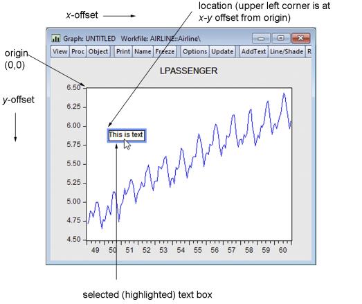
To place text within a graph, you can use explicit coordinates to specify the position of the upper left corner of the text.
Coordinates are set by a pair of numbers
h,
v in virtual inches. Individual graphs are always

virtual inches (scatter diagrams are

virtual inches) or a user-specified size, regardless of their current display size.
The origin of the coordinate is the upper left hand corner of the graph. The first number h specifies how many virtual inches to offset to the right from the origin. The second number v specifies how many virtual inches to offset below the origin. The upper left hand corner of the text will be placed at the specified coordinate.
Coordinates may be used with other options, but they must be in the first two positions of the options list. Coordinates are overridden by other options that specify location.
When addtext is used with a multiple graph, the text is applied to the whole graph, not to each individual graph.
Color definitions
color_arg specifies the color to be employed in the arguments above. The color may be specified using predefined color names, by specifying the individual red-green-blue (RGB) components using the special “@RGB” function, or by specifying the individual red-green-blue (RGB) components in hexadecimal using the special “@HEX” function.
The predefined colors are given by the keywords (with their RGB and HEX equivalents):
blue | @rgb(0, 0, 255) | @hex(0000ff) |
red | @rgb(255, 0, 0) | @hex(ff0000) |
ltred | @rgb(255, 168, 168) | @hex(ffa8a8) |
green | @rgb(0, 128, 0) | @hex(008000) |
black | @rgb(0, 0, 0) | @hex(000000) |
white | @rgb(255, 255, 255) | @hex(ffffff) |
purple | @rgb(128, 0, 128) | @hex(800080) |
orange | @rgb(255, 128, 0) | @hex(ff8000) |
yellow | @rgb(255, 255, 0) | @hex(ffff00) |
gray | @rgb(128, 128, 128) | @hex(808080) |
ltgray | @rgb(192, 192, 192) | @hex(c0c0c0) |
Examples
freeze(g1) gdp.line
g1.addtext(t) "Fig 1: Monthly GDP (78m1-95m12)"
places the text “Fig1: Monthly GDP (78m1-95m12)” centered above the graph G1.
g1.addtext(.2, .2, X) "Seasonally Adjusted"
places the text “Seasonally Adjusted” in a box within the graph, slightly indented from the upper left corner.
g1.addtext(t, x, textcolor(red), fillcolor(128,128,128), framecolor(black)) "Civilian\rUnemployment (First\\Last)"
adds the text “Civilian Unemployment (First\Last)” where there is a return between the “Civilian” and “Unemployment”. The text is colored red, and is enclosed in a gray box with a black frame.
Cross-references
Align placement of multiple graphs.
Syntax
graph_name.align(n,h,v)
Options
You must specify three numbers (each separated by a comma) in parentheses in the following order: the first number n is the number of columns in which to place the graphs, the second number h is the horizontal space between graphs, and the third number v is the vertical space between graphs. Spacing is specified in virtual inches.
Examples
mygraph.align(3,1.5,1)
aligns MYGRAPH with graphs placed in three columns, horizontal spacing of 1.5 virtual inches, and vertical spacing of 1 virtual inch.
var var1.ls 1 4 m1 gdp
freeze(impgra) var1.impulse(m,24) gdp @ gdp m1
impgra.align(2,1,1)
estimates a VAR, freezes the impulse response functions as multiple graphs, and realigns the graphs. By default, the graphs are stacked in one column, and the realignment places the graphs in two columns.
Cross-references
For a detailed discussion of customizing graphs, see
“Graphing Data”.
Sets axis scaling and display characteristics for the graph.
By default, EViews optimally chooses the axis scaling to fit the graph data.
Syntax
graph_name.axis(axis_id) options_list
The axis_id parameter identifies which of the axes the command modifies. If no option is specified, the proc will modify all of the axes. axis_id may take on one of the following values:
left / l | Left vertical axis. |
right / r | Right vertical axis. |
bottom / b | Bottom axis for XY and scatter graphs (
scat,
xyarea,
xybar,
xyline,
xypair). |
top / t | Top axis for XY and scatter graphs (
scat,
xyarea,
xybar,
xyline,
xypair). |
zerotop / zeroback | Draw zero line on [top / bottom] of other graph elements. |
all / a | All axes. |
Options
The options list may include any of the following options:
Data scaling options
linear | Linear data scaling (default). |
linearzero | Linear data scaling (include zero when auto range selection is employed). |
log | Logarithmic scaling. |
norm | Norm (standardize) the data prior to plotting. |
range(arg) | Specifies the endpoints for the scale, where arg may be: “auto” (automatic choice), “minmax” (use the maximum and minimum values of the data), “n1, n2” (set minimum to n1 and maximum to n2, e.g. “range(3, 9)”). |
overlap / ‑overlap | [Overlap / Do not overlap] scales on dual scale graphs. |
invert / -invert | [Invert / do not invert] scale. |
units(arg) | Specifies the units of the data, where arg may be: “n” (native), “p” (percent), “k” (thousands), “m” (millions), “b” (billions), “t” (trillions). |
format(option1 [,option2, ...]) | Sets data formatting, where you may provide one or more of the following options:
“commadec” / “-commadec” ([Do / Do not] use comma as decimal, “ksep” / “-ksep” ([Do / Do not] include a thousands separator, “leadzero” / “-leadzero” ([Do / Do not] include leading zeros, “dec=arg” (set number of decimal places, where arg may be an integer or “a” for auto), “prefix=c” (add a prefix character, where c may be a single quoted character or “” to remove the prefix), “suffix=c” (add a suffix character, where c may be a single quoted character or “” to remove the suffix). |
Axis options
grid / -grid | [Draw / Do not draw] grid lines. |
zeroline /
‑zeroline | [Draw / Do not draw] a line at zero on the data scale. |
zerotop /
-zerotop | [Draw / Do not draw] the zero line on top of the graph. |
ticksout | Draw tickmarks outside the graph axes. |
ticksin | Draw tickmarks inside the graph axes. |
ticksboth | Draw tickmarks both outside and inside the graph axes. |
ticksnone | Do not draw tickmarks. |
ticksauto | Allow EViews to determine whether to draw tickmarks on or between observations. |
tickson | Draw tickmarks on observations. |
ticksbtw | Draw tickmarks between observations. |
ticksbtwns | Draw tickmarks between observations, removing space at the axis ends. |
minor / -minor | [Allow / Do not allow] minor tick marks. |
label / -label | [Place / Do not place] labels on the axes. |
duallevel / -duallevel | [Allow / Do not allow] two row date labels on the observation axis. |
font([face], [pt], [+/- b], [+/- i], [+/- u], [+/- s]) | Set characteristics of axis font. The font name (face), size (pt), and characteristics are all optional. face should be a valid font name, enclosed in double quotes. pt should be the font size in points. The remaining options specify whether to turn on/off boldface (b), italic (i), underline (u), and strikeout (s) styles. |
textcolor(arg) | Sets the color of the axis text. arg may be one of the predefined color keywords, or it may be specified using individual red-green-blue (RGB) components using the “@RGB” or “@HEX” functions. The arguments to the @RGB function are a set of three integers from 0 to 255, representing the RGB values of the color. The arguments to the “@HEX” function are a set of six characters representing the RGB values of the color in hexadecimal. Each two character set represents a red, green or blue component in the range '00' to 'FF'. For a description of the available color keywords see
“Color definitions”. |
mirror / -mirror | [Label / Do not label] both left and right axes with duplicate axes (single scale graphs only). |
angle(arg) | Set label angle, where arg can be an integer between -90 and 90 degrees, measured in 15 degree increments, or “a” (auto) for automatically determined angling. The angle is measured from the horizontal axis. |
The options which support the “–” may be preceded by a “+” or “–” indicating whether to turn on or off the option. The “+” is optional.
Note that the default settings are taken from the Global Defaults.
Color definitions
color_arg specifies the color to be employed in the arguments above. The color may be specified using predefined color names, by specifying the individual red-green-blue (RGB) components using the special “@RGB” function, or by specifying the individual red-green-blue (RGB) components in hexadecimal using the special “@HEX” function.
The predefined colors are given by the keywords (with their RGB and HEX equivalents):
blue | @rgb(0, 0, 255) | @hex(0000ff) |
red | @rgb(255, 0, 0) | @hex(ff0000) |
ltred | @rgb(255, 168, 168) | @hex(ffa8a8) |
green | @rgb(0, 128, 0) | @hex(008000) |
black | @rgb(0, 0, 0) | @hex(000000) |
white | @rgb(255, 255, 255) | @hex(ffffff) |
purple | @rgb(128, 0, 128) | @hex(800080) |
orange | @rgb(255, 128, 0) | @hex(ff8000) |
yellow | @rgb(255, 255, 0) | @hex(ffff00) |
gray | @rgb(128, 128, 128) | @hex(808080) |
ltgray | @rgb(192, 192, 192) | @hex(c0c0c0) |
Examples
To set the right scale to logarithmic with manual range, you can enter:
graph1.axis(right) log range(10, 30)
graph1.axis(r) zeroline -minor font(12)
draws a horizontal line through the graph at zero on the right axis, removes minor ticks, and changes the font size of the right axis labels to 12 point.
graph2.axis -mirror
turns of mirroring of axes in single scale graphs.
mygra1.axis font("Times", 12, b, i) textcolor(blue)
sets the axis font to blue “Times” 12pt bold italic.
gra1.axis(l) units(b) format(ksep, prefix="$", suffix="")
plots the data on the left axis in billions, using commas to separate thousands, adds a “$” to the beginning of each data label and erases the suffix.
Cross-references
See
“Graph Objects” for a discussion of graph options.
Specify labeling of a boxplot axis.
Note that
bplabel is no longer supported. See instead,
Graph::setobslabel.
Clear the contents of the history attribute for graph objects.
Removes the graph’s history attribute, as shown in the label view of the graph.
Syntax
graph_name.clearhist
Examples
g1.clearhist
g1.label
The first line removes the history from the graph G1, and the second line displays the label view of G1, including the now blank history field.
Cross-references
See
“Labeling Objects” for a discussion of labels and display names.
Clear the contents of the remarks attribute.
Removes the graph’s remarks attribute, as shown in the label view of the graph.
Syntax
graph_name.clearremarks
Examples
g1.clearremarks
g1.label
The first line removes the remarks from the graph G1, and the second line displays the label view of G1, including the now blank remarks field.
Cross-references
See
“Labeling Objects” for a discussion of labels and display names.
Creates a copy of the graph.
Creates either a named or unnamed copy of the graph.
Syntax
graph_name.copy
graph_name.copy dest_name
Examples
g1.copy
creates an unnamed copy of the graph G1.
g1.copy g2
creates G2, a copy of the graph G1.
Cross-references
Control labeling of the data points in graphs.
datelabel sets options that are control the labeling of individual data points in graphs
Syntax
graph_name.datalabel option_list
Options
pos(arg) | Label position relative to the data point on the graph. The following positions are available: L – Left of point (vertically centered) R – Right of point (vertically centered) A – Above the point (horizontally centered) B – Below the point (horizontally centered) C – Centered on pointed (vertically and horizontally) Auto – Auto position |
point(arg) | Which data points to label, where arg can be: All – label all data points First – label only the first visible data point Last – label only the last visible data point |
label(arg) | Specifies the contents of the label, where arg is the custom label string containing text and keywords. The following keywords are replaced with their appropriate values: @legend – the legend label of the series @xlabel – the x-axis label of the data point @ylabel – the y-axis label of the data point |
color(arg) | The label text color. Use ‘none’ to set the text color as black. Nothing specified will set the text color to match the line color. If the color option is not specified, the color will be unchanged. |
point(arg) | Which data points to label, where arg can be: All – label all data points First – label only the first visible data point Last – label only the last visible data point |
Examples
graph1.datalabel point(first) pos(r) label(Start of recession\n(@xlabel(), @ylabel())) color()
will label the first data point of all the series in graph1. The label will be located to the right of the data point. The label will contain the 2 line string where the first line will read “Start of recession” and the second line will contain the comma separated x-value and y-value of the first data point enclosed in parenthesis (example: “(1948Q4,1.1)”). The label color will match the line color.
graph2.datalabel point(all) pos(a) label((@xlabel():@ylabel())) color(none)
will label all of the data points in graph2. The labels will appear above the associated data points in black and will be of the form “(x-value:y-value)” (example: “(1976:900.3)”).
graph3.datalabel point(last) pos(l) label(@legend()-@ylabel()) color()
will label all the series in graph3 but only the last data point for each series. The labels will appear the left of the associated data points and will be of the form “legend label-y-value” (example: “Nevada-35.6”). The label color will match the line color.
Cross-references
Control labeling of the bottom date/time axis in time plots.
datelabel sets options that are specific to the appearance of time/date labeling. Many of the options that also affect the appearance of the date axis are set by the
Graph::axis command with the “bottom” option. These options include tick control, label and font options, and grid lines.
Syntax
graph_name.datelabel option_list
Options
format("datestring") | datestring should be one of the supported data formats describing how the date should appear. The datestring argument should be enclosed in double-quotes. For example, “yy:mm” specifies two-digit years followed by a colon delimited and then two-digit months. You may use the special single space datestring “ “ to indicate automatic formatting. You may also add “\n” to denote a new line providing the option to make the date string 2 lines. For example, “Month\nyear” will place the month on the first line and the year on the second. Note: there is a 2 line maximum. A second “\n” will therefore create an error. EViews provides considerable flexibility in formatting your dates. See
“Date Formats” for a complete description. |
interval(step_size [,steps][,align_date]) | where step_size takes one of the following values: “auto” (steps and align_date are ignored), “ends” (only label endpoints; steps and align_date are ignored), “all” (label every point; the steps and align_date options are ignored), “obs” (steps are one observation), “year” (steps are one year), “m” (steps are one month), “q” (steps are one quarter). steps is a number (default=1) indicating the number of steps between labels. align_date is a date specified to receive a label. Note, the align_date should be in the units of the data being graphed, but may lie outside the current sample or workfile range. |
span(arg) | Specify date label spanning: “auto” (automatic determination), “on” (turn spanning on; label start of period, tick on obs.), “between” (center label on period), “trimbetween” (center label on period, trim spaces at axis ends). Consider the case of a yearly label with monthly ticks. If span is on, the label is centered on the 12 monthly ticks. If the span option is off, year labels are put on the first quarter or month of the year. |
end / -end | [Use / Do not use] end-of-period labeling. |
duallevel / -duallevel | [Allow / Do not allow] two row date labels on the observation axis. |
Examples
graph1.datelabel format(yyyy:mm)
will display dates using four-digit years followed by the default delimiter “:” and a two-digit month (e.g. – “1974:04”).
graph1.datelabel format(yy[q]mm)
will display a two-digit year followed by a “q” separator and then a two-digit month (e.g. – “74q04”)
graph1.datelabel interval(y, 2, 1951)
specifies labels every two years on odd numbered years.
graph1.datelabel format(“Month dd\nYYYY”)
specifies time axis label will have 2 lines. The first line will contain the full month name and day and the second line will contain the 4 digit year.
Cross-references
See
“Graph Objects” for a discussion of graph options.
See the replacement command
Graph::datelabel.
Removes all objects of specified type from a graph object.
Syntax
graph_name.delete object_type
where object_type includes one or more of the following: ‘line’, ‘shade’, ‘text’, ‘ellipse’, ‘rectangle’, and ‘arrow’.
Examples
The following removes all line and shade objects from GRA1
gra1.delete line shade
To remove all text objects from GRA1:
gra1.delete text
Cross-references
Display table, graph, or spool output in the graph object window.
Display the contents of a table, graph, or spool in the window of the graph object.
Syntax
graph_name.display object_name
Examples
graph1.display tab1
Display the contents of the table TAB1 in the window of the object GRAPH1.
Cross-references
See
“Labeling Objects” for a discussion of labels and display names.
Display name for a graph object.
Attaches a display name to a graph object which may be used to label output in place of the standard graph object name.
Syntax
graph_name.displayname display_name
Display names are case-sensitive, and may contain a variety of characters, such as spaces, that are not allowed in graph object names.
Examples
gr1.displayname Hours Worked
gr1.label
The first line attaches a display name “Hours Worked” to the graph GR1, and the second line displays the label view of GR1, including its display name.
Cross-references
See
“Labeling Objects” for a discussion of labels and display names.
Place horizontal or vertical lines and shaded areas on the graph.
Syntax
graph_name.draw(draw_type, axis_id [,options]) position [position2]
where draw_type may be one of the following:
line / l | A line |
shade | A shaded area |
Note that the “dashline” option has been removed (though it is supported for backward compatibility). You should use the “pattern” option to specify whether the line is solid or patterned.
axis_id may take the values:
left / l | Draw a horizontal line or shade using the left axis to define the drawing position |
right / r | Draw a horizontal line or shade using the right axis to define the drawing position |
bottom / b | Draw a vertical line or shade using the bottom axis to define the drawing position |
If drawing a line, the drawing position is taken from position. If drawing a shaded area, you can either specify a start and end position (position and position2), sample object, or sample string to define the boundaries of the shaded region.
Line/Shade Options
The following options may be provided to change the characteristics of the specified line or shade. Any unspecified options will use the default text settings of the graph.
color(arg) | Specifies the color of the line or shade. arg may be one of the predefined color keywords, or it may be specified using individual red-green-blue (RGB) components using the “@RGB” or “@HEX” functions. The arguments to the @RGB function are a set of three integers from 0 to 255, representing the RGB values of the color. The arguments to the “@HEX” function are a set of six characters representing the RGB values of the color in hexadecimal. Each two character set represents a red, green or blue component in the range '00' to 'FF'. For a description of the available color keywords see
“Color definitions”. The default is black for lines and gray for shades. RGB values may be examined by calling up the color palette in the dialog. |
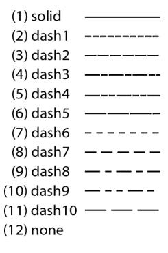
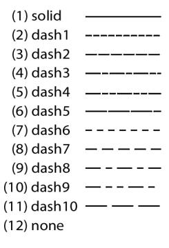
pattern(index) | Sets the line pattern to the type specified by index. index can be an integer from 1 to 12 or one of the matching keywords (“solid”, “dash1” through “dash10”, “none”). The “none” keyword turns on solid lines. |
width(n1) | Specify the width, where n1 is the line width in points (used only if object_type is “line” or “dashline”). The default is 0.5 points. |
top | Specifies that the line be drawn on top of the graph. (Note that this option has no effect on shades.) |
Color definitions
color_arg specifies the color to be employed in the arguments above. The color may be specified using predefined color names, by specifying the individual red-green-blue (RGB) components using the special “@RGB” function, or by specifying the individual red-green-blue (RGB) components in hexadecimal using the special “@HEX” function.
The predefined colors are given by the keywords (with their RGB and HEX equivalents):
blue | @rgb(0, 0, 255) | @hex(0000ff) |
red | @rgb(255, 0, 0) | @hex(ff0000) |
ltred | @rgb(255, 168, 168) | @hex(ffa8a8) |
green | @rgb(0, 128, 0) | @hex(008000) |
black | @rgb(0, 0, 0) | @hex(000000) |
white | @rgb(255, 255, 255) | @hex(ffffff) |
purple | @rgb(128, 0, 128) | @hex(800080) |
orange | @rgb(255, 128, 0) | @hex(ff8000) |
yellow | @rgb(255, 255, 0) | @hex(ffff00) |
gray | @rgb(128, 128, 128) | @hex(808080) |
ltgray | @rgb(192, 192, 192) | @hex(c0c0c0) |
Examples
graph1.draw(line, left, @rgb(0,0,255)) 5.25
draws a horizontal blue line at the value “5.25” as measured on the left axis while:
graph1.draw(shade, right) 7.1 9.7
draws a shaded horizontal region bounded by the right axis values “7.1” and “9.7”. You may also draw vertical regions by using the “bottom” axis_id:
graph1.draw(shade, bottom) 1980:1 1990:2
draws a shaded vertical region bounded by the dates “1980:1” and “1990:2”.
graph1.draw(shade, bottom, @rgb(255,0,0)) 1980:1 1990:2 if x>.5
draws red shaded vertical regions bounded by the dates “1980:1” and “1990:2” where the series x has a value greater than .5.
graph1.draw(shade, bottom, @rgb(0,128,0)) mysample
draws green shaded vertical regions that match the mysample object.
graph1.draw(line, bottom, pattern(dash1)) 1985:1
draws a vertical dashed line at “1985:1”.
Cross-references
See
“Graph Objects” for a discussion of graph options.
See
Graph::drawdefault for setting defaults.
Change default settings for lines and shaded areas in the graph.
This command specifies changes in the default settings which will be applied to line and shade objects added subsequently to the graph. If you include the “existing” option, all of the drawing default settings will also be applied to existing line and shade objects in the graph.
Syntax
graph_name.drawdefault draw_options
where draw_options may include one or more of the following:
linecolor(arg) | Sets the default color for lines. arg may be one of the predefined color keywords, or it may be specified using individual red-green-blue (RGB) components using the “@RGB” or “@HEX” functions. The arguments to the @RGB function are a set of three integers from 0 to 255, representing the RGB values of the color. The arguments to the “@HEX” function are a set of six characters representing the RGB values of the color in hexadecimal. Each two character set represents a red, green or blue component in the range '00' to 'FF'. For a full description of the keywords, see
“Color definitions”. |
shadecolor(arg) | Sets the default color for shades. arg may be one of the predefined color keywords, or it may be specified using individual red-green-blue (RGB) components using the “@RGB” or “@HEX” functions. The arguments to the @RGB function are a set of three integers from 0 to 255, representing the RGB values of the color. The arguments to the “@HEX” function are a set of six characters representing the RGB values of the color in hexadecimal. Each two character set represents a red, green or blue component in the range '00' to 'FF'. For a full description of the keywords, see
“Color definitions” |
width(n1) | Specify the width, where n1 is the line width in points (used only if object_type is “line” or “dashline”). The default is 0.5 points. |
pattern(index) | Sets the default line pattern to the type specified by index. index can be an integer from 1 to 12 or one of the matching keywords (“solid”, “dash1” through “dash10”, “none”). Sets the line pattern to the type specified by index. index can be an integer from 1 to 12 or one of the matching keywords (“solid”, “dash1” through “dash10”, “none”). The “none” keyword turns on solid lines. |
existing | Apply the default settings to all existing line/shade objects in the graph. |
Color definitions
color_arg specifies the color to be employed in the arguments above. The color may be specified using predefined color names, by specifying the individual red-green-blue (RGB) components using the special “@RGB” function, or by specifying the individual red-green-blue (RGB) components in hexadecimal using the special “@HEX” function.
The predefined colors are given by the keywords (with their RGB and HEX equivalents):
blue | @rgb(0, 0, 255) | @hex(0000ff) |
red | @rgb(255, 0, 0) | @hex(ff0000) |
ltred | @rgb(255, 168, 168) | @hex(ffa8a8) |
green | @rgb(0, 128, 0) | @hex(008000) |
black | @rgb(0, 0, 0) | @hex(000000) |
white | @rgb(255, 255, 255) | @hex(ffffff) |
purple | @rgb(128, 0, 128) | @hex(800080) |
orange | @rgb(255, 128, 0) | @hex(ff8000) |
yellow | @rgb(255, 255, 0) | @hex(ffff00) |
gray | @rgb(128, 128, 128) | @hex(808080) |
ltgray | @rgb(192, 192, 192) | @hex(c0c0c0) |
Examples
graph1.drawdefault linecolor(blue) width(.25) existing
changes the default setting for new line/shade objects. New lines added to the graph will now be drawn in blue, with a width of 0.25 points. In addition, all existing line and shade objects will be updated with the graph default settings. Note that in addition to the line color and width settings specified in the command, the existing default line pattern and shade colors will be applied to the line and shade objects in graph.
graph1.drawdefault existing
updates all line and shade objects in the graph with the currently specified default draw object settings.
Cross-references
See
“Graph Objects” for a discussion of graph options.
Create named graph object containing the results of a graph command, or created when merging multiple graphs into a single graph.
Syntax
graph graph_name.graph_command(options) arg1 [arg2 arg3 ...]
graph graph_name.merge graph1 graph2 [graph3 ...]
Follow the keyword with a name for the graph, a period, and then a statement used to create a graph. There are two distinct forms of the command.
In the first form of the command, you create a graph using one of the graph commands, and then name the object using the specified name. The portion of the command given by,
graph_command(options) arg1 [arg2 arg3 ...]
should follow the form of one of the standard EViews graph commands:
area | |
band | |
bar | |
boxplot | Boxplot graph (
boxplot). |
distplot | Distribution graph (
distplot). |
dot | |
errbar | Error bar graph (
errbar). |
hilo | High-low(-open-close) graph (
hilo). |
line | |
pie | |
qqplot | Quantile-Quantile graph (
qqplot). |
scat | Scatterplot—same as XY, but lines are initially turned off, symbols turned on, and a  frame is used (
scat). |
scatmat | Matrix of scatterplots (
scatmat). |
scatpair | Scatterplot pairs graph (
scatpair). |
seasplot | Seasonal line graph (
seasplot). |
spike | |
xyarea | XY line-symbol graph with one X plotted against one or more Y’s using existing line-symbol settings (
xyarea). |
xybar | XY line-symbol graph with one X plotted against one or more Y’s using existing line-symbol settings (
xybar). |
xyline | Same as XY, but symbols are initially turned off, lines turned on, and a  frame is used (
xyline). |
xypair | Same as XY but sets XY settings to display pairs of X and Y plotted against each other (
xypair). |
In the second form of the command, you instruct EViews to merge the listed graphs into a single graph, and then name the graph object using the specified name.
Options
reset | Resets all graph options to the global defaults. May be used to remove existing customization of the graph. |
p | Print the graph (for use when specified with a graph command). |
Additional options will depend on the type of graph chosen. See the entry for each graph type for a list of the available options (for example, see
bar for details on bar graphs).
Examples
graph gra1.line(s, p) gdp m1 inf
creates and prints a stacked line graph object named GRA1. This command is equivalent to running the command:
line(s, p) gdp m1 inf
freezing the view, and naming the graph GRA1.
graph mygra.merge gr_line gr_scat gr_pie
creates a multiple graph object named MYGRA that merges three graph objects named GR_LINE, GR_SCAT, and GR_PIE.
Cross-references
See
“Graph Objects” for a general discussion of graphs.
Display or change the label view of a graph object, including the last modified date and display name (if any).
As a procedure, label changes the fields in the graph label.
Syntax
graph_name.label
graph_name.label(options) [text]
Options
The first version of the command displays the label view of the graph. The second version may be used to modify the label. Specify one of the following options along with optional text. If there is no text provided, the specified field will be cleared.
c | Clears all text fields in the label. |
d | Sets the description field to text. |
s | Sets the source field to text. |
u | Sets the units field to text. |
r | Appends text to the remarks field as an additional line. |
p | Print the label view. |
Examples
The following lines replace the remarks field of GRA1 with “Data from CPS 1988 March File”:
gra1.label(r)
gra1.label(r) Data from CPS 1988 March File
To append additional remarks to GRA1, and then to print the label view:
gra1.label(r) Log of hourly wage
gra1.label(p)
To clear and then set the units field, use:
gra1.label(u) Millions of bushels
Cross-references
See
“Labeling Objects” for a discussion of labels.
Set legend appearance and placement in graphs.
When
legend is used with a multiple graph, the legend settings apply to all graphs. See
Graph::setelem for setting legends for individual graphs in a multiple graph.
Syntax
graph_name.legend option_list
Options
columns(arg) (default=“auto”) | Columns for legend: “auto” (automatically choose number of columns), int (put legend in specified number of columns). |
display/–display | Display/do not display the legend. |
inbox/–inbox | Put legend in box/remove box around legend. |
position(arg) | Position for legend: “left” or “l” (place legend on left side of graph), “right” or “r” (place legend on right side of graph), “botleft” or “bl” (place left-justified legend below graph), “botcenter” or “bc” (place centered legend below graph), “botright” or “br” (place right-justified legend below graph), “(h, v)” (the first number h specifies the number of virtual inches to offset to the right from the origin. The second number v specifies the virtual inch offset below the origin. The origin is the upper left hand corner of the graph). |
font([face], [pt], [+/- b], [+/- i], [+/- u], [+/- s]) | Set characteristics of legend font. The font name (face), size (pt), and characteristics are all optional. face should be a valid font name, enclosed in double quotes. pt should be the font size in points. The remaining options specify whether to turn on/off boldface (b), italic (i), underline (u), and strikeout (s) styles. |
textcolor(arg) | Sets the color of the legend text. arg may be one of the predefined color keywords, or it may be specified using individual red-green-blue (RGB) components using the “@RGB” or “@HEX” functions. The arguments to the @RGB function are a set of three integers from 0 to 255, representing the RGB values of the color. The arguments to the “@HEX” function are a set of six characters representing the RGB values of the color in hexadecimal. Each two character set represents a red, green or blue component in the range '00' to 'FF'. For a description of the available color keywords see
“Color definitions”. |
fillcolor(arg) | Sets the background fill color of the legend box. arg may be one of the predefined color keywords, or it may be specified using individual red-green-blue (RGB) components using the “@RGB” or “@HEX” functions. The arguments to the @RGB function are a set of three integers from 0 to 255, representing the RGB values of the color. The arguments to the “@HEX” function are a set of six characters representing the RGB values of the color in hexadecimal. Each two character set represents a red, green or blue component in the range '00' to 'FF'. For a description of the available color keywords see
“Color definitions”. |
framecolor(arg) | Sets the color of the legend box frame. arg may be one of the predefined color keywords, or it may be specified using individual red-green-blue (RGB) components using the “@RGB” or “@HEX” functions. The arguments to the @RGB function are a set of three integers from 0 to 255, representing the RGB values of the color. The arguments to the “@HEX” function are a set of six characters representing the RGB values of the color in hexadecimal. Each two character set represents a red, green or blue component in the range '00' to 'FF'. For a description of the available color keywords see
“Color definitions”. |
The options which support the “–” may be preceded by a “+” or “–” indicating whether to turn on or off the option. The “+” is optional.
The default settings are taken from the global defaults.
Color definitions
color_arg specifies the color to be employed in the arguments above. The color may be specified using predefined color names, by specifying the individual red-green-blue (RGB) components using the special “@RGB” function, or by specifying the individual red-green-blue (RGB) components in hexadecimal using the special “@HEX” function.
The predefined colors are given by the keywords (with their RGB and HEX equivalents):
blue | @rgb(0, 0, 255) | @hex(0000ff) |
red | @rgb(255, 0, 0) | @hex(ff0000) |
ltred | @rgb(255, 168, 168) | @hex(ffa8a8) |
green | @rgb(0, 128, 0) | @hex(008000) |
black | @rgb(0, 0, 0) | @hex(000000) |
white | @rgb(255, 255, 255) | @hex(ffffff) |
purple | @rgb(128, 0, 128) | @hex(800080) |
orange | @rgb(255, 128, 0) | @hex(ff8000) |
yellow | @rgb(255, 255, 0) | @hex(ffff00) |
gray | @rgb(128, 128, 128) | @hex(808080) |
ltgray | @rgb(192, 192, 192) | @hex(c0c0c0) |
Examples
mygra1.legend display position(l) inbox
places the legend of MYGRA1 in a box to the left of the graph.
mygra1.legend position(.2,.2) -inbox
places the legend of MYGRA1 within the graph, indented slightly from the upper left corner with no box surrounding the legend text.
mygra1.legend font("Times", 12, b, i) textcolor(red) fillcolor(blue) framecolor(blue)
sets the legend font to red “Times” 12pt bold italic, and changes both the legend fill and frame colors to blue.
Cross-references
See
“Graph Objects” for a discussion of graph objects in EViews.
See
Graph::addtext and
Graph::textdefault. See
Graph::setelem for changing legend text and other graph options.
Creates a group object containing all the series in the graph.
Syntax
graph_name.makegroup group_name
group_name is an optional new group name. Group will be untitled if group_name is not specified.
Examples
mygraph.makegroup mynewgroup
Creates new group called mynewgroup.
mygraph.makegroup
Creates an untitled group.
Merge graph objects.
merge combines graph objects into a single graph object. The graph objects to merge must exist in the current workfile.
Syntax
graph_name.merge graph1 graph2 [graph3 ...]
Follow the keyword with a list of existing graph object names to merge.
Examples
graph mygra.merge gra1 gra2 gra3 gra4
show mygra.align(4,1,1)
The first line merges the four graphs GRA1, GRA2, GRA3, GRA4 into a graph named MYGRA. The second line displays the four graphs in MYGRA in a single row.
Cross-references
See
“Graph Objects” for a discussion of graphs.
Save graph to disk as an enhanced or ordinary Windows metafile.
Provided for backward compatibility,
metafile has been replaced by the more general graph proc
Graph::save, which allows for saving graphs in metafile or postscript files, with additional options for controlling the output.
Change the names used for legends or axis labels in XY graphs.
Allows you to provide an alternative to the names used for legends or for axis labels in XY graphs. The name command is available only for single graphs and will be ignored in multiple graphs.
Syntax
graph_name.name(n) legend_text
Provide a series number in parentheses and legend_text for the legend (or axis label) after the keyword. If you do not provide text, the current legend will be removed from the legend/axis label.
Examples
graph g1.line(d) unemp gdp
g1.name(1) Civilian unemployment rate
g1.name(2) Gross National Product
The first line creates a line graph named G1 with dual scale, no crossing. The second line replaces the legend of the first series UNEMP, and the third line replaces the legend of the second series GDP.
graph g2.scat id w h
g2.name(1)
g2.name(2) weight
g2.name(3) height
g2.legend(l)
The first line creates a scatter diagram named G2. The second line removes the legend of the horizontal axis, and the third and fourth lines replace the legends of the variables on the vertical axis. The last line moves the legend to the left side of the graph.
Cross-references
See
“Graph Objects” for a discussion of working with graphs.
Push updates to OLE linked objects in open applications.
Syntax
graph_name.olepush
Cross-references
See
“Object Linking and Embedding (OLE)” for a discussion of using OLE with EViews.
Set options for a graph object.
Allows you to change the option settings of an existing graph object. When options is used with a multiple graph, the options are applied to all graphs.
Syntax
graph_name.options option_list
Options
Basic Graph Options
legend / -legend | Turn on and off legend. |
size(w, h) | Specifies the size of the plotting frame in virtual inches (w=width, h=height). |
lineauto | Use solid lines when drawing in color and use patterns and grayscale when drawing in black and white. |
linesolid | Always use solid lines. |
linepat | Always use line patterns. |
color / -color | Specifies that lines/filled areas [use / do not use] color. Note that if the “lineauto” option is specified, this choice will also influence the type of line or filled area drawn on screen: if color is specified, solid colored lines and filled areas will be drawn; if color is turned off, lines will be drawn using black and white line patterns, and gray scales will be used for filled areas. |
barlabelabove /
-barlabelabove | [Place / Do not place] text value of data above bar in bar graph. |
barlabelinside barlabelinside | [Place / Do not place] text value of data inside bar in bar graph. |
barlabelnone | Remove text value of data from bar graph. |
outlinebars /
-outlinebars | [Outline / Do not outline] bars in a bar graph. |
outlinearea /
-outlinearea | [Outline / Do not outline] areas in an area graph. |
outlineband /
-outlineband | [Outline / Do not outline] bands in an area band graph. |
barspace /‑barspace | [Put / Do not put] space between bars in bar graph. |
pielabel /
-pielabel | [Place / Do not place] text value of data in pie chart. |
automult/-automult | [Auto reduce / Do not autoreduce] frame size in multiple graphs to make text appear larger |
dual/-dual | [Overlap / Do not overlap] scales (no cross). |
barfade(arg) | Sets the fill fade of the bars in a bar graph. arg may be: “none” (solid fill - default), “3d” (3D rounded fill), “lzero” (light at zero), “dzero” (dark at zero). |
antialias(arg) | Sets anti-aliasing to smooth the appearance of data lines in the graph. arg may be: “auto” (EViews uses anti-aliasing where appropriate - default), “on”, or “off”. |
interpolate(arg) | Sets the interpolation method to estimate values between two known data points in the graph. arg may be: “linear” (no interpolation), “mild” (mild spline), “medium” (medium spline), or “full” (full spline). |
stackposneg / ‑stackposneg | For bar graphs, stack positive and negative values separately (Excel style). |
Graph Grid Options
gridl / -gridl | [Turn on / Turn off] grid lines on the left scale. |
gridr / -gridr | [Turn on / Turn off] grid lines on the right scale. |
gridb / -gridb | [Turn on / Turn off] grid lines on the bottom scale. |
gridt / -gridt | [Turn on / Turn off] grid lines on the top scale. |
gridnone | No grid lines (turns of time scale grid). |
gridauto | Allow EViews to place grid lines at automatic intervals. |
gridcust(freq [,step]) | Place grid lines at custom intervals, specified by freq. freq may be: “obs” or “o” (Step = One obs), “year” or “y” (Step = Year), “quarter” or “q” (Step = Quarter), “month” or “m” (Step = Month), “day” or “d” (Step = Day), “user” or “u” (Step = custom). You may optionally specify a step for the interval. If not specified, the default is the last grid step used for this graph, or 1 if a step has never been specified. |
gridcolor(arg) | Sets the grid line color. arg may be one of the predefined color keywords, or it may be specified using individual red-green-blue (RGB) components using the “@RGB” or “@HEX” functions. The arguments to the @RGB function are a set of three integers from 0 to 255, representing the RGB values of the color. The arguments to the “@HEX” function are a set of six characters representing the RGB values of the color in hexadecimal. Each two character set represents a red, green or blue component in the range '00' to 'FF'. For a description of the available color keywords see
“Color definitions”. |
gridwidth(n) | Sets the width of the grid lines in points. n should be a number between 0.25 and 5. |
gridpat(index) | Sets the default line pattern to the type specified by index. index can be an integer from 1 to 12 or one of the matching keywords (“solid”, “dash1” through “dash10”, “none”). Sets the line pattern to the type specified by index. index can be an integer from 1 to 12 or one of the matching keywords (“solid”, “dash1” through “dash10”, “none”). The “none” keyword turns on solid lines. |
gridontop /
-gridontop | [Draw / Do not draw] the grid lines on top of the graph. |
Background and Frame Options
fillcolor(arg) | Sets the fill color of the graph frame. arg may be one of the predefined color keywords, or it may be specified using individual red-green-blue (RGB) components using the “@RGB” or “@HEX” functions. The arguments to the @RGB function are a set of three integers from 0 to 255, representing the RGB values of the color. The arguments to the “@HEX” function are a set of six characters representing the RGB values of the color in hexadecimal. Each two character set represents a red, green or blue component in the range '00' to 'FF'. For a description of the available color keywords see
“Color definitions”. |
backcolor(arg) | Sets the background color of the graph. arg may be one of the predefined color keywords, or it may be specified using individual red-green-blue (RGB) components using the “@RGB” or “@HEX” functions. The arguments to the @RGB function are a set of three integers from 0 to 255, representing the RGB values of the color. The arguments to the “@HEX” function are a set of six characters representing the RGB values of the color in hexadecimal. Each two character set represents a red, green or blue component in the range '00' to 'FF'. For a description of the available color keywords see
“Color definitions”. |
framecolor(arg) | Sets the background color of the graph frame. arg may be one of the predefined color keywords, or it may be specified using individual red-green-blue (RGB) components using the “@RGB” or “@HEX” functions. The arguments to the @RGB function are a set of three integers from 0 to 255, representing the RGB values of the color. The arguments to the “@HEX” function are a set of six characters representing the RGB values of the color in hexadecimal. Each two character set represents a red, green or blue component in the range '00' to 'FF'. For a description of the available color keywords see
“Color definitions”.. |
fillfade(arg) | Sets the fill fade of the graph frame. arg may be: “none” (solid frame fill - default), “ltop” (light at top), “dtop” (dark at top). |
backfade(arg) | Sets the background fade of the graph. arg may be: “none” (solid background - default), “ltop” (light at top), “dtop” (dark at top). |
framewidth(n) | Sets the width of the graph frame in points. n should be a number between 0.25 and 5. |
frameaxes(arg) | Specifies which frame axes to display. arg may be one of the keywords: “all”, “none”, or “labeled” (all axes that have labels), or any combination of letters “l” (left), “r” (right), “t” (top), and “b” (bottom), e.g. “lrt” for left, right and top. |
indenth(n) | Sets the horizontal indentation of the graph from the graph frame in virtual inches. n should be a number between 0 and 0.75. |
indentv(n) | Sets the vertical indentation of the graph from the graph frame in virtual inches. n should be a number between 0 and 0.75. |
inbox / -inbox | [Show / Do not show] the graph frame on axes that do not have data assigned to them. |
background / ‑background | [Include / Do not include] the background color when exporting or printing the graph. |
Sample Break and NA Handling
drop (default) | For a graph with a non-contiguous sample, drop the excluded observations from the graph scale. |
connect | For a graph with missing values or a non-contiguous sample, connect non-missing observations. |
disconnect | For a graph with missing values or a non-contiguous sample, disconnect non-missing observations. |
pad | For a graph with a non-contiguous sample, pad the graph scale with the excluded observations |
segment | For a graph with a non-contiguous sample, drop the excluded observations from the graph scale and draw vertical lines at the seams in the observation scale. |
The options which support the “–” may be preceded by a “+” or “–” indicating whether to turn on or off the option. The “+” is optional.
Data labels in bar and pie graphs will only be visible when there is sufficient space in the graph.
Color definitions
color_arg specifies the color to be employed in the arguments above. The color may be specified using predefined color names, by specifying the individual red-green-blue (RGB) components using the special “@RGB” function, or by specifying the individual red-green-blue (RGB) components in hexadecimal using the special “@HEX” function.
The predefined colors are given by the keywords (with their RGB and HEX equivalents):
blue | @rgb(0, 0, 255) | @hex(0000ff) |
red | @rgb(255, 0, 0) | @hex(ff0000) |
ltred | @rgb(255, 168, 168) | @hex(ffa8a8) |
green | @rgb(0, 128, 0) | @hex(008000) |
black | @rgb(0, 0, 0) | @hex(000000) |
white | @rgb(255, 255, 255) | @hex(ffffff) |
purple | @rgb(128, 0, 128) | @hex(800080) |
orange | @rgb(255, 128, 0) | @hex(ff8000) |
yellow | @rgb(255, 255, 0) | @hex(ffff00) |
gray | @rgb(128, 128, 128) | @hex(808080) |
ltgray | @rgb(192, 192, 192) | @hex(c0c0c0) |
Examples
graph1.options size(4,4) +inbox color
sets
GRAPH1 to use a

frame enclosed in a box. The graph will use color.
graph1.options linepat -color size(2,8) -inbox
sets GRAPH1 to use a

frame with no box. The graph does not use color, with the lines instead being displayed using patterns.
graph1.options fillcolor(gray) backcolor(192, 192, 192) framecolor(blue)
sets the fill color of the graph frame to gray, the background color of the graph to the RGB values 192, 192, and 192, and the graph frame color to blue.
graph1.options gridpat(3) gridl -gridb
display left scale grid lines using line pattern 3 (“dash2”) and turn off display of vertical grid lines from the bottom axis.
graph1.options indenth(.5) frameaxes(lb) framewidth(.5) gridwidth(.25)
indents the graph .5 virtual inches from the frame, displays left and bottom frame axes of width .5 points, and sets the gridline width to .25 points.
Cross-references
See
“Graph Objects” for a discussion of graph options in EViews.
Save a graph object to disk as a Windows metafile (.EMF or .WMF), PostScript (.EPS), bitmap (.BMP), Graphics Interchange Format (.GIF), Joint Photographic Experts Exchange (.JPEG), Portable Network Graphics (.PNG), Portable Document Format (.PDF), LaTeX (.TEX), Markdown (.MD), or MPEG-4 (.mp4).
Syntax
graph_name.save(options) [path\]file_name
Follow the keyword with a name for the file. file_name may include the file type extension, or the file type may be specified using the “t=” option. A graph may be saved with an EMF, WMF, EPS, BMP, GIF, JPG, PNG, PDF, TEX, MD, or MP4 extension. The MD (Markdown) setting uses very basic syntax and should be usable in most editors.
If an explicit path is not specified, the file will be stored in the default directory, as set in the global options.
Graph Options
t=file_type | Specifies the file type, where file_type may be one of: Enhanced Windows metafile (“emf” or “meta”), ordinary Windows metafile (“wmf”), Encapsulated PostScript (“eps” or “ps”), Bitmap file (“bmp”), Graphics Interchange Format (“gif”), Joint Photographic Experts Exchange (“jpeg” or “jpg”), Portable Network Graphics (“png”), Portable Document Format (“pdf”), LaTeX (“tex”), Markdown (“md”), or MPEG-4 (“mp4”). Files will be saved with the “.emf”, “.wmf”, “.eps”, “.bmp”, “.gif”, “.jpeg”, “.png”, “.pdf”, “.tex”, “.md”, or “.mp4” extensions, respectively. |
u=units | Specify units of measurement, where units is one of: “in” (inches), “cm” (centimeters), “pt” (points), “pica” (picas), “pixels” (pixels). Note: pixels are only applicable to bmp, gif, jpeg, and png files. Default is inches otherwise. |
w=width | Set width of the graphic in the selected units. |
h=height | Set height of the graphic in the selected units. |
c / -c | [Save / Do not save] the graph in color. |
trans / -trans | [Set / Do not set] background to transparent (for graph formats which support transparency). |
d = dpi | Specify the number of dots per inch. Only applicable to bmp, gif, jpeg, and png files when units has not been set to pixels. In the case units = “pixels”, it is ignored. |
Note that if only a width or a height option is specified, EViews will calculate the other dimension holding the aspect ratio of the graph constant. If both width and height are provided, the aspect ratio will no longer be locked. (Note that the aspect ratio for an ordinary Windows Metafile (.WMF) cannot be unlocked, so only a height or width should be specified in this case.) EViews will default to the current graph dimensions if size is unspecified.
All defaults with exception to dots per inch are taken from the global graph export settings (Options/Graphics Defaults.../Exporting). The default dots per inch for bmp, gif, jpeg, and png file types is equal to the number of pixels per logical inch along the screen width of your system. Values may therefore differ from system to system.
Postscript Options
box / -box | [Save / Do not save] the graph with a bounding box. The bounding box is an invisible rectangle placed around the graphic to indicate its boundaries. The default is taken from the global graph export settings. |
land | Save the graph in landscape orientation. The default uses portrait mode. |
prompt | Force the dialog to appear from within a program. |
LaTeX Options
texspec / -texspec | [Include / Do not include] the full LaTeX documentation specification in the LaTeX output. The default behavior is taken from the global default settings. |
Examples
graph1.save(t=ps, -box, land) c:\data\MyGra1
saves GRAPH1 as a PostScript file MYGRA1.EPS. The graph is saved in landscape orientation without a bounding box.
graph2.save(t=emf, u=pts, w=300, h=300) MyGra2
saves GRAPH2 in the default directory as an Enhanced Windows metafile MYGRA2.EMF. The image will be scaled to

points.
graph3.save(t=png, u=in, w=5, d=300) MyGra3
saves GRAPH3 in the default directory as a PNG file MYGRA3.PNG. The image will be 5 inches wide at 300 dpi.
Cross-references
See
“Graph Objects” for a discussion of graphs.
The
scale command is supported for backward compatibility, but has been replaced by the
Graph::axis command, which handles all axis and scaling options.
Set the object attribute.
Syntax
graph_name.setattr(attr) attr_value
Sets the attribute attr to attr_value. Note that quoting the arguments may be required. Once added to an object, the attribute may be extracted using the @attr data member.
Examples
a.setattr(revised) never
String s = a.@attr("revised")
sets the “revised” attribute in the object A to the string “never”, and extracts the attribute into the string object S.
Cross-references
Enable/disable individual boxplot elements.
Syntax
graph_name.setbpelem element_list
The element_list may contain one or more of the following:
median, med / -median, -med | [Show / Do not show] the medians. |
mean / -mean | [Show / Do not show] the means. |
whiskers, w / -whiskers, -w | [Show / Do not show] the whiskers (lines from the box to the staples). |
staples, s / -staples, -s | [Show / Do not show] the staples (lines drawn at the last data point within the inner fences). |
near / -near | [Show /Do not show] the near outliers (values between the inner and outer fences). |
far / -far | [Show / Do not show] the far outliers (values beyond the outer fences). |
width(arg) (default =“fixed”) | Set the width settings for the boxplots, where arg is one of: “fixed” (uniform width), “n” (proportional to sample size), “rootn” (proportional to the square root of sample size). |
ci(arg) (default= “shade”) | Set the display method for the median confidence intervals, where arg is one of: “none” (do not display), “shade” (shaded intervals), “notch” (notched intervals). |
Examples
graph01.setbpelem -far width(n) ci(notch)
hides the far outliers, sets the box widths proportional to the number of observations, and enables notching of the confidence intervals.
Cross-references
See
“Boxplot” for a description of boxplots.
See
Graph::setelem to modify line and symbol attributes. See also
Graph::options and
Graph::axis.
Set individual line, bar and legend options for each series in the graph.
Syntax
graph_name.setelem(graph_elem) argument_list
where graph_elem is the identifier for the graph element whose options you wish to modify:
integer | Index for graph element (for non-boxplot graphs). For example, if you provide the integer “2”, EViews will modify the second line in the graph. |
box_elem | Boxplot element to be modified: box (“b”), median (“med”), mean (“mean”), near outliers (“near” or “no”), far outliers (“far” or “fo”), whiskers (“w”), staples (“s”). For boxplot graphs only. |
The argument list for setelem may contain one or more of the following:
symbol(arg) | Sets the drawing symbol: arg can be an integer from 1–18, or one of the matching keywords. “obslabel” and “dotobslabel”, and “dotobslabelcircle” use the observation label as the symbol. Selecting a symbol automatically turns on symbol use. The “none” option turns off symbol use. |
symbolsize(arg), symsize(arg) | Sets the symbol size. arg may be an integer between 1-8, where 1 is the smallest symbol and 8 is the largest, or one of the keywords: “XS” (X-Small), “S” (Small), “M” (Medium), “L” (Large), “XL” (X-Large), “2XL” (2X-Large), “3XL” (3X-Large), “4XL” (4X-Large). |
linecolor(arg), lcolor(arg) | Sets the line and symbol color. arg may be one of the predefined color keywords, or it may be specified using individual red-green-blue (RGB) components using the “@RGB” or “@HEX” functions. The arguments to the @RGB function are a set of three integers from 0 to 255, representing the RGB values of the color. The arguments to the “@HEX” function are a set of six characters representing the RGB values of the color in hexadecimal. Each two character set represents a red, green or blue component in the range '00' to 'FF'. For a description of the available color keywords see
“Color definitions”. |
linewidth(n1), lwidth(n1) | Sets the line and symbol width: n1 should be a number between “.25” and “5”, indicating the width in points. |
linepattern(arg), lpat(arg) | Sets the line pattern to the type specified by arg. arg can be an integer from 1–12 or one of the matching keywords. Note that the option interacts with the graph options for “color”, “lineauto”, “linesolid”, “linepat” (see
Graph::options, for details). You may need to set the graph option for “linepat” to enable the display of line patterns. See
Graph::options. Note also that the patterns with index values 7–11 have been modified since version 5.0. In particular, the “none” option has been moved to position 12. The “none” option turns off lines and uses only symbols. |
lineopacity(arg1[, arg2]) | Sets the line opacity to the value or setting specified by the arg values. The arg can be an value from 0 to 1, or one of the keywords “auto”, “on”, “off”. If the opacity setting currently “on” or “auto” (default), setting the level to 0.0 will make (in relevant cases) the object completely transparent (0% opacity) while a value of 1.0 will make the object completely opaque (100% opacity). Setting opacity to “off” will make the object fully opaque. |
fillcolor(arg), fcolor(arg) | Sets the fill color for symbols, bars, and pies. arg may be one of the predefined color keywords, or it may be specified using individual red-green-blue (RGB) components using the “@RGB” function or “@HEX” functions. The arguments to the @RGB function are a set of three integers from 0 to 255, representing the RGB values of the color. The arguments to the “@HEX” function are a set of six characters representing the RGB values of the color in hexadecimal. Each two character set represents a red, green or blue component in the range '00' to 'FF'. For a description of the available color keywords see
“Color definitions”. |
fillgray(n1), gray(n1) | Sets the gray scale for bars and pies: n1 should be an integer from 1–15 corresponding to one of the predefined gray scale settings (from lightest to darkest). |
fillhatch(arg), hatch(arg) | Sets the hatch characteristics for bars and pies: arg can be an integer from 1–7, or one of the matching keywords. |
fillopacity(arg1[, arg2]), | Sets the fill opacity to the opacity to the value or setting specified by the arg values. The arg can be an value from 0 to 1, or one of the keywords “auto”, “on”, “off”. If the opacity setting currently “on” or “auto” (default), setting the level to 0.0 will make (in relevant cases) the object completely transparent (0% opacity) while a value of 1.0 will make the object completely opaque (100% opacity). Setting opacity to “off” willmake the object fully opaque. |
preset(n1) | Sets line and fill characteristics to the specified EViews preset values, where n1 is an integer from 1–30. Simultaneously sets “linecolor”, “linepattern”, “linewidth”, “symbol”, “fillcolor”, “fillgray”, and “fillhatch” to the EViews predefined definitions for graph element n1. When applied to boxplots, the line color of the specified element will be applied to the box, whiskers, and staples. |
default(n1) | Sets line and fill characteristics to the specified user-defined default settings where n1 is an integer from 1–30. Simultaneously sets “linecolor”, “linepattern”, “linewidth”, “symbol”, “fillcolor”, “fillgray”, and “fillhatch” to the values in the user-defined global defaults for graph element n1. When applied to boxplots, the line color of the specified settings will be applied to the box, whiskers, and staples. |
axis(arg), scale(arg) | Assigns the element to an axis: left (“l”), right (“r”), bottom (“b”), top (“t”). The latter two options are only applicable for XY and scatter graphs (
scat,
xyarea,
xybar,
xyline,
xypair). |
legend(str) | Assigns legend text for the element. str will be used in the legend to label the element. |
Color definitions
color_arg specifies the color to be employed in the arguments above. The color may be specified using predefined color names, by specifying the individual red-green-blue (RGB) components using the special “@RGB” function, or by specifying the individual red-green-blue (RGB) components in hexadecimal using the special “@HEX” function.
The predefined colors are given by the keywords (with their RGB and HEX equivalents):
blue | @rgb(0, 0, 255) | @hex(0000ff) |
red | @rgb(255, 0, 0) | @hex(ff0000) |
ltred | @rgb(255, 168, 168) | @hex(ffa8a8) |
green | @rgb(0, 128, 0) | @hex(008000) |
black | @rgb(0, 0, 0) | @hex(000000) |
white | @rgb(255, 255, 255) | @hex(ffffff) |
purple | @rgb(128, 0, 128) | @hex(800080) |
orange | @rgb(255, 128, 0) | @hex(ff8000) |
yellow | @rgb(255, 255, 0) | @hex(ffff00) |
gray | @rgb(128, 128, 128) | @hex(808080) |
ltgray | @rgb(192, 192, 192) | @hex(c0c0c0) |
Examples
graph1.setelem(2) lcolor(blue) lwidth(2) symbol(circle)
sets the second line of GRAPH1 to be a blue line of width 2 with circle symbols.
graph1.setelem(1) lcolor(blue)
graph1.setelem(1) linecolor(0, 0, 255)
are equivalent methods of setting the linecolor to blue.
graph1.setelem(1) fillgray(6)
sets the gray-scale color for the first graph element.
The lines:
graph1.setelem(1) scale(l)
graph1.setelem(2) scale(l)
graph1.setelem(3) scale(r)
create a dual scale graph where the first two series are scaled together and labeled on the left axis, and the third series is scaled and labeled on the right axis.
graph1.setelem(2) legend("gross domestic product")
sets the legend for the second graph element.
Cross-references
See
“Graph Objects” for a discussion of graph options in EViews.
Set the font for text in the graph.
Syntax
graph_name.setfont font_args
The font_args may include one or more of the following:
type([face], [pt], [+/- b], [+/- i], [+/- u], [+/- s]) | Set characteristics of the font for the graph element type. The font name (face), size (pt), and characteristics are all optional. face should be a valid font name, enclosed in double quotes. pt should be the font size in points. The remaining options specify whether to turn on/off boldface (b), italic (i), underline (u), and strikeout (s) styles. |
and type is one of “all”, “axes”, “legend”, “text”, “obs”, where “axes” refers to the axes labels, “legend” refers to the graph legend, “text” refers to the added text, “obs” refers to the observation scale, and “all” refers to all of the elements.
Examples
mygraph.setfont axes("Times", 20, b)
sets the font to Times, 20pt, bold for all of the graph elements.
mygraph.setfont text("Arial") legend("Helvetica")
sets the added text font to Arial and the legend font to Helvetica.
Cross-references
See
“Graph Objects” for a discussion of graph options.
Sets custom axis labels for the observation scale of a graph.
Syntax
graph_name.setobslabel([step_options,] init_options) [string1 string2 ...]
Follow the keyword with a list of axis labels, or the name of a series when the “series” init_option is used.
To preserve case, enclose the label in quotation marks. To hide a label, use “”. If the number of labels provided is less than the number of existing labels, the remaining labels will not be affected.
Options
Step options
start[, step] | start should be the observation number of the first label to modify. step defines the number of observations to skip between applying labels. |
Init options
init_options (default = “blank”) | init_options sets initialization options for the labels. For a frozen graph (updating off), you may use the keywords: “current” (keep current labels, or initialize the labels with standard observation labels if custom labels do not currently exist, then add the labels provided), “obsnum” (initialize with observation numbers), or “blank” (set all labels to empty strings, then add the labels provided). For live or frozen graphs, you may use the keywords: “series” (initialize the labels with the values of a series; follow the command with the name of a series instead of labels), or “clear” (delete custom labels if they exist and return to automatic labeling). |
Examples
Given a graph GRA1 with updating turned off, change the first label to “CA” using the command:
gra1.setobslabel(current) "CA"
Note that all but the first label remain unchanged.
To keep the first label as “CA” and set the second label to “OR”, you could enter:
gra1.setobslabel(current) "CA" "OR"
Alternatively, an equivalent command would be
gra1.setobslabel(2,current) "OR"
which starts applying labels at the second observation.
To set the first, third, and fifth observation labels in the frozen graph GRAPH2 and leave all others unchanged:
graph2.setobslabel(1,2,current) "first" "third" "fifth"
This instructs EViews to begin modifying at the first label and step two observations between new labels.
graph2.setobslabel(1,2,blank) "first" "third" "fifth"
performs the same operation as the previous command, while also clearing out all other labels.
graph2.setobslabel(clear)
deletes all custom labels and returns to EViews automatic labeling.
Say we have an alpha series in our workfile, ALPHA01, whose values are: “CA”, “OR”, “WA”, etc. To use these values as axis labels, use the series option and specify a series name in place of labels:
gra3.setobslabel(series) alpha01
This command creates labels on the time axis, using values in ALPHA01 to label the observations with: “CA”, “OR”, “WA”, etc.
Cross-references
See
“Graph Objects” for a discussion of graph options.
Set the update state of a graph object.
Syntax
graph_name.setupdate(options) [sample]
Follow the name of the graph with a period, the keyword setupdate, and the update setting.
Optionally, include a sample with the “manual” or “automatic” options to restrict updates to data changes made within the sample period. If you do not include a sample, updates will occur according to changes in the workfile sample.
Options
“off” or “o” | Turn updating off. |
“manual” or “m” | Update when requested (with the
Graph::update command), or when the graph type is changed. |
“auto” or “a” | Update whenever the update condition is met. If a sample is specified, an update will occur when data changes within the sample. If no sample is specified, updates will occur when data or the workfile sample changes. |
Examples
gr1.setupdate(o)
This command turns off updating for graph GR1.
gr1.setupdate(a)
turns on automatic updating for graph GR1, according to the workfile sample. Whenever the underlying data or the workfile sample changes, GR1 will be updated with the changes.
gr2.setupdate(m) 1992 1993
turns on manual updating for graph GR2, for the sample period 1992 to 1993. When the graph is manually updated, using the
update command, changes in data between 1992 and 1993 will be updated.
Cross-references
See
“Graph Objects” for a discussion of graph updating options.
Sort the series in a graph.
The sort command sorts all series in the graph on the basis of the values of up to three series. For purposes of sorting, NAs are considered to be smaller than any other value. By default, EViews will sort the series in ascending order. You may use options to override the sort order.
Note that sorting cannot be undone. You may wish to freeze or copy the graph before applying the sort.
Syntax
graph_name.sort(series1[, series2, series3])
Follow the keyword with a list of the series by which you wish to sort the graph. If you list two or more series, sort uses the values of the second series to resolve ties from the first series, and values of the third series to resolve ties from the second.
The series may be specified using the series display name or the index of the series in the graph. For example, if you provide the integer “2”, EViews will use the second series. To sort by observation labels, use the integer “0” or the keyword “Obs label”.
To sort in descending order, precede the series name with a minus sign (“-”).
Note that a graph with more than 500 observations cannot be sorted.
Examples
gra1.sort(x,y)
sorts graph GRA1 first by the series X. Any ties in X will be resolved by the series Y.
If X is the first series in graph GRA1 and Y is the second series,
gra1.sort(1,-2)
sorts first in ascending order by X and then in descending order by Y.
gra1.sort(0)
sorts GRA1 by its observation labels.
Apply a template to a graph object.
If you apply template to a multiple graph object, the template options will be applied to each graph in the multiple graph. If the template graph is a multiple graph, the options of the first graph will be used.
Syntax
graph_name.template(options) template
Follow the name of the graph to which you want to apply the template options with a period, the keyword template, and the name of a graph template. template may be one of the predefined template keywords: “default” (current global defaults), “classic”, “modern”, “reverse”, “midnight”, “spartan”, “monochrome”, or a named graph in the workfile.
Options
t | Replace text and line/shade objects with those of the template graph, when template is the name of a graph in the workfile. |
e | Apply template settings to existing text and line/fill options. |
b / -b | [Apply / Remove] bold modifiers of the specified predefined template style. |
w / -w | [Apply / Remove] wide modifiers of the specified predefined template style. |
axis / -axis | [Apply / Remove] axis modifiers of the specified template. |
legend / -legend | [Apply / Remove] legend modifiers of the specified template. |
The options which support the “–” may be preceded by a “+” or “–” indicating whether to turn on or off the option. The “+” is optional.
Examples
gra_cs.template gra_gdp
applies the option settings in the graph object
GRA_GDP to the graph
GRA_CS. Text and line shading options from GRA_GDP will be applied to GRA_CS, but the characteristics of existing text and line/shade objects in GRA_CS will not be modified. Text and shading objects include those added with the
Graph::addtext or
Graph::draw commands.
g1.template(t) mygraph1
applies the option settings of MYGRAPH1, and all text and shadings in the template graph, to the graph G1. Note that the “t” option overwrites any existing text and shading objects in the target graph.
graph1.template(e) modern
applies the predefined template “modern” to GRAPH1, also changing the settings of existing text and line/shade objects in the graph.
graph1.template(e, b, w) reverse
applies the predefined template “reverse” to GRAPH1, with the bold and wide modifiers. Any existing text and line/shade objects in GRAPH1 are also modified to use the object settings of the monochrome template.
graph1.template(-w) monochrome
applies the monochrome settings to GRAPH1, removing the wide modifier.
If you are using a boxplot as a template for another graph type, or vice versa, note that the graph types and boxplot specific attributes will not be changed. In addition, when the “t” option is used, vertical lines or shaded areas will not be copied between the graphs, since the horizontal scales differ.
Cross-references
See
“Templates” for additional discussion.
Change default settings for text objects in the graph.
This command specifies changes in the default settings which will be applied to text objects added subsequently to the graph. If you include the “existing” option, all of the text default settings will also be applied to existing text objects in the graph.
Syntax
graph_name.textdefault text_options
where text_options include one or more of one of the following:
font([face], [pt], [+/- b], [+/- i], [+/- u], [+/- s]) | Set characteristics of default text font. The font name (face), size (pt), and characteristics are all optional. face should be a valid font name, enclosed in double quotes. pt. should be the font size in points. The remaining options specify whether to turn on/off boldface (b), italic (i), underline (u), and strikeout (s) styles. |
textcolor(arg) | Sets the default color of the text. arg may be one of the predefined color keywords, or it may be specified using individual red-green-blue (RGB) components using the “@RGB” or “@HEX” functions. The arguments to the @RGB function are a set of three integers from 0 to 255, representing the RGB values of the color. The arguments to the “@HEX” function are a set of six characters representing the RGB values of the color in hexadecimal. Each two character set represents a red, green or blue component in the range '00' to 'FF'. For a description of the available color keywords see
“Color definitions”. |
fillcolor(arg) | Sets the default background fill color of the text box. arg may be one of the predefined color keywords, or it may be specified using individual red-green-blue (RGB) components using the “@RGB” or “@HEX” functions. The arguments to the @RGB function are a set of three integers from 0 to 255, representing the RGB values of the color. The arguments to the “@HEX” function are a set of six characters representing the RGB values of the color in hexadecimal. Each two character set represents a red, green or blue component in the range '00' to 'FF'. For a description of the available color keywords see
“Color definitions”. |
framecolor(arg) | Sets the default color of the text box frame. arg may be one of the predefined color keywords, or it may be specified using individual red-green-blue (RGB) components using the “@RGB” or “@HEX” functions. The arguments to the @RGB function are a set of three integers from 0 to 255, representing the RGB values of the color. The arguments to the “@HEX” function are a set of six characters representing the RGB values of the color in hexadecimal. Each two character set represents a red, green or blue component in the range '00' to 'FF'. For a description of the available color keywords see
“Color definitions”. |
existing | Apply the default settings to all existing text objects in the graph. |
The options which support the “–” may be preceded by a “+” or “–” indicating whether to turn on or off the option. The “+” is optional.
Color definitions
color_arg specifies the color to be employed in the arguments above. The color may be specified using predefined color names, by specifying the individual red-green-blue (RGB) components using the special “@RGB” function, or by specifying the individual red-green-blue (RGB) components in hexadecimal using the special “@HEX” function.
The predefined colors are given by the keywords (with their RGB and HEX equivalents):
blue | @rgb(0, 0, 255) | @hex(0000ff) |
red | @rgb(255, 0, 0) | @hex(ff0000) |
ltred | @rgb(255, 168, 168) | @hex(ffa8a8) |
green | @rgb(0, 128, 0) | @hex(008000) |
black | @rgb(0, 0, 0) | @hex(000000) |
white | @rgb(255, 255, 255) | @hex(ffffff) |
purple | @rgb(128, 0, 128) | @hex(800080) |
orange | @rgb(255, 128, 0) | @hex(ff8000) |
yellow | @rgb(255, 255, 0) | @hex(ffff00) |
gray | @rgb(128, 128, 128) | @hex(808080) |
ltgray | @rgb(192, 192, 192) | @hex(c0c0c0) |
Examples
graph1.textdefault font("Arial", b) fillcolor(gray) framecolor(@rgb(0,0,255)) existing
changes the default text settings for new text objects so that new text is in Arial bold, using the current default font size and color. Should the new text be enclosed in a box, the box will have a gray fill and blue frame color. Additionally, the “existing” keyword specifies that existing text objects in the graph will be updated with the current text settings. Note that in addition to the font type and fill color specified in the command, all text default settings will be applied to the existing text.
graph1.textdefault existing
updates the text objects in GRAPH1 with the current text default settings.
Cross-references
See
“Graph Objects” for a discussion of graph options.
Update graph.
This command updates a graph that has updating turned on.
Syntax
graph_name.update
Examples
graph1.update
If GRAPH1 is a graph with manual updating enabled, this command instructs the graph to update its data. If the graph has automatic updating enabled, this command is unnecessary, as it will simply repeat the automatic update. For a graph with updating off, this command does nothing.
Cross-references
See
“Graph Objects” for a discussion of graph updating options.