Econometrics and Statistics
EViews 12 offers a exciting new additions and improvements to its set of econometric and statistical features. The following is a brief outline of the most important new features, followed by additional discussion and pointers to full documentation.
Regression Variable Selection
Variable selection, or feature selection as it is sometimes called in computer science literature, is an important component of modern machine learning. EViews includes three such techniques: Stepwise, and (new to EViews 12) Lasso and Auto-Search/GETS.
Each of these techniques are implemented in EViews as a pre-estimation step before performing a standard least squares regression. Before estimation, you must specify a dependent variable together with a list of always-included variable, and a list of selection variables, from which the selection algorithm will choose the most appropriate. Following the variable selection process, EViews reports the results of the final regression
•
“Auto-Search / GETS” offers an improvement of stepwise regression techniques by adding tests of model validity to the selection process.
•
“Lasso” outlines how the Lasso estimation technique, which is based on estimating regression where the objective penalizes complexity, may be also used as a pre-estimation tool to determine the regressors in least squares.
Indicator Saturation
EViews 12 adds regression tools for testing outliers and structural breaks in a regression specification based on the indicator saturation approach.
The indicator saturation approach is an extension of least squares regression for testing for outliers and structural breaks in a regression specification. The indicator saturation approach works by including indicator variables for outliers or structural breaks at every observation in the regression, and then employing the GETS algorithms to select which of the included variables should be retained in a final regression model.
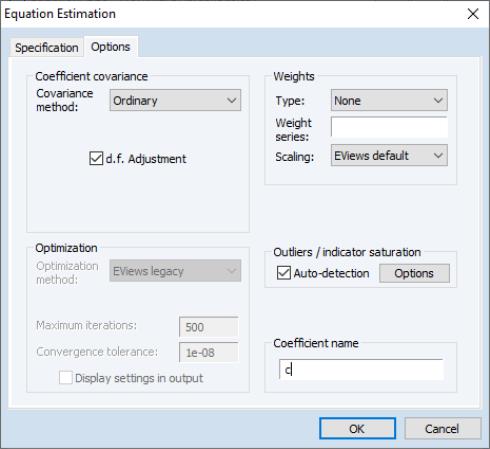
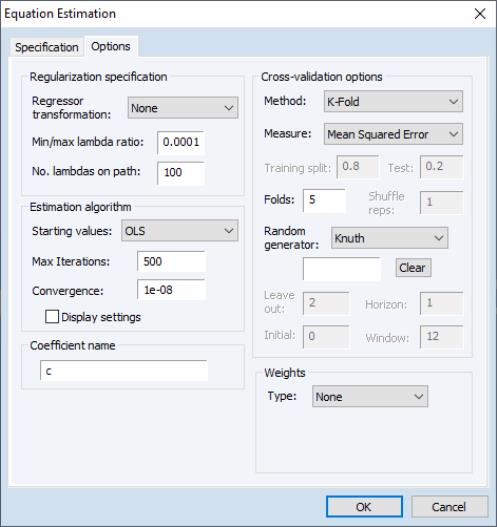
To instruct EViews to detect indicators in your least squares regression, open the equation estimation dialog, enter your least squares specification in the edit field, and select in the dialog. Next, click on the Options tab to display the dialog:
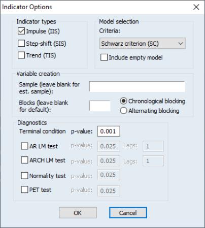
Select the check box in thearea on the right-hand side of the dialog, and then press the tab to bring up the dialog:
Mixed-Frequency Regression
Mixed Data Sampling (MIDAS) regression was introduced in EViews in earlier versions. MIDAS is an estimation technique which allows for data sampled at different frequencies to be used in the same regression.
More specifically, the MIDAS methodology (Ghysels, Santa-Clara, and Valkanov, (2002) and Gyhsels, Santa-Clara, and Valkanaov (2006), and Andreou, Ghysels, and Kourtellos (2010)) addresses the situation where the dependent variable in the regression is sampled at a lower frequency than one or more of the regressors. The goal of the MIDAS approach is to incorporate the information in the higher frequency data into the lower frequency regression in a parsimonious, yet flexible fashion.
EViews 12 extends the existing MIDAS toolbox by adding additional estimation options. These new features allow you to use the General-to-Specific (GETS) method for variable selection and indicator saturation.
See
“Midas Regression” for additional discussion.
See also
Equation::midas for command documentation.
FI(E)GARCH and GARCH Tools
EViews 12 introduces several new tools for estimating and working with conditional variance models. These tools include new estimation methods that allow for long-memory processes, and new equation views that make it easy to examine the properties of your GARCH estimated equations:
• FIGARCH / FIEGARCH.
• News Impact, Stability Tests, Sign Bias Misspecification tests.
FI(E)GARCH
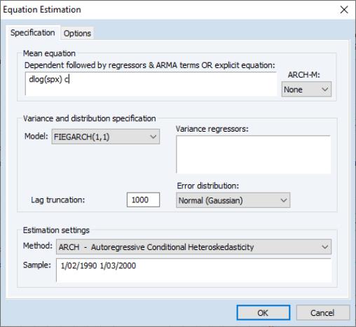
EViews 12 estimates Fractionally Integrated GARCH (FIGARCH) models, with support for both standard FIGARCH and Fractionally Integrated Exponential GARCH (FIEGARCH) specifications.
While traditional GARCH models focus on short term dynamics of conditional variance, the fractionally integrated GARCH model (FIGARCH) model, introduced by Baillie, Bollerslev and Mikkelsen (1996, BBM), is designed to capture long run dependence properties of the variance. The FIEGARCH model of Bollerslev and Mikkelsen (1996) adds FIGARCH long-memory innovations to EGARCH processes.
News Impact, Stability Tests, Sign Bias Misspecification Tests
In addition, EViews 12 offers three new views for all GARCH models.
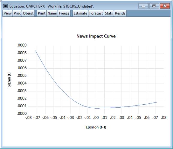
News Impact Curve
A news impact curve plots the change in the conditional volatility against a change (or shock) in past news.
Specifically, the news impact curve uses the estimated GARCH equation specification to plot values of the conditional volatility

against

, while setting

for

, and holding all lagged

for

constant at the unconditional variance.
To display a news impact curve, select GARCH Graphs/News Impact Curve from the view menu of an estimated GARCH equation.
News impact curves are not available for fractionally integrated GARCH models.
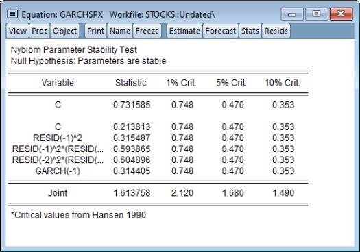
Stability Tests
The Nyblom Stability Test is a test of parameter stability or structural change. The test provides individual statistics on each parameter (both in the mean and variance equations) and a joint test of null hypothesis is that the parameters are constant through time.
To compute the test, select from the menu of an equation estimated by GARCH:
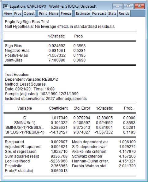
Sign Bias Misspecification Tests
The Sign Bias Test (Engle and Ng, 1993) provides a test for misspecification of the conditional variance model. The test performs a regression of the squared residuals against dummy variables based upon the sign previous residuals. If a GARCH model is correctly specified, the sign of previous residuals should have no impact upon the current squared residuals. The null hypothesis is that the parameters of the regression are zero.
To conduct the test, select from the menu of an equation estimated by GARCH:
Elastic Net and Lasso
Elastic net regularization is a popular solution to the overfitting problem, where a model fits training data well but does not generalize easily to new test data. Depending on the particular parameters chosen for the elastic net model, some or all of the regressors are preserved, but their magnitudes are reduced.
EViews 11 includes tools for estimation of elastic net, ridge, and Lasso regression models. EViews supports estimation over a single lambda penalization parameter and a grid search over multiple penalization parameters. When multiple parameters are used, EViews also supports options for automatic generation of penalization parameters, as well as cross-validation tools for choosing the parameter with the lowest error.
EViews 12 offer a number of additions to the existing toolkit:
• new cross-validation options for selecting penalty function including rolling and expanding window methods for selecting training and test sets.
• new diagnostics showing training-test set cross-validation composition.
• estimation with observation and variable weights.
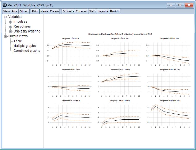
Impulse Response User Interface
EViews 12 features a new interface for computing and displaying impulse responses and confidence intervals for VAR and VEC estimators.
The prior impulse response interface coupled the choices for which impulses and responses to display and the method in which they were displayed, with the various options for computing the impulse response and standard error. Thus, if a user first displayed a multiple graph of impulse responses and then wanted to show the results in a table, or perhaps display a subset of those original responses, the procedure would have to be respecified and recomputed from the beginning.
The new, dynamic EViews 12 interface allows for interactive selection of the impulse and responses to be displayed, as well as the method of display. This flexibility is particularly important in light of the introduction of new, computationally intensive, VAR and VEC bootstrap confidence interval evaluation methods (
“Bootstrap Impulse Response Confidence Intervals”).Bootstrap Impulse Response Confidence Intervals
EViews 12 introduces several new bootstrapping approaches to computing the confidence intervals for both VAR and VEC impulse responses.
These new tools allow you to compute residual bootstrap, residual double bootstrap, and fast residual double bootstrap estimates of these confidence intervals. EViews supports a variety of confidence interval bootstrap methods, including standard percentile, Hall’s (1992) percentile confidence intervals, Hall’s (1986) studentized confidence interval, and Killian’s (1998) unbiased confidence interval.
Panel and Pool Two-way Cluster Robust Covariances
In many settings, observations may be grouped into different groups or “clusters” where errors are correlated for observations in the same cluster and uncorrelated for observations in different clusters. This cluster error correlation must be accounted for in computing estimates of the precision of regression estimates.
In a panel equation and pool settings, versions of EViews prior to EViews 12 offered tools for computing coefficient covariances accounting for clusters defined by cross-section units or by periods. Following the lead of the system estimation literature, these robust standard error calculations were termed “White cross-section” for clustering by period, to indicate that there was contemporaneous correlation between cross-section units, and termed “White period” for clustering by cross-section, to indicate that there was between period correlation within a cross-section unit.
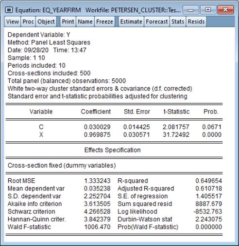
EViews 12 extends these tools to allow for computation of robust covariances when clusters are defined by both cross-section units and periods (Petersen 2009, Thompson 2011, Cameron, Gelbach, and Miller 2015).
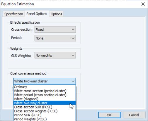
To estimate a two-way cluster robust coefficient covariance in EViews, open the equation dialog in your panel workfile, then click on the tab to display the panel equations options page:
In the method combo on the left, select for one-way period clustering, for one-way cross-section clustering, for unstructured heteroskedasticity robust covariances, or for clustering by both cross-section and period.
Click on to estimate the equation with this option and display the estimation results.
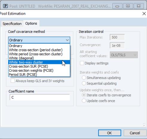
You may also compute two-way clustered standard errors in pooled data settings. Simply open the pool object, click on , and then on the tab:
Note that to support these new features, panel equations and pools with cluster robust or PCSE and TCSE standard errors estimated by EViews 12 are not backward compatible with earlier versions of EViews.
Functional Coefficients Models
Functional coefficient regression is a semi-parametric approach to extend the standard regression framework by allowing the

to be functions of the variable

(Fan and Gijbels (1996); Cai, Fan, and Yao (2000)).
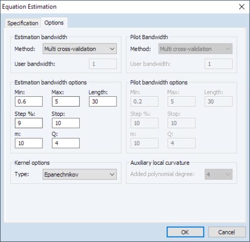
EViews 12 offers a completely revamped interface for estimating and working with these models along with new tools for examining the properties of your functional coefficients estimates:
• Enhanced Interface provides additional control over the computation of final and pilot bandwidths, with new methods for obtaining bandwidths.
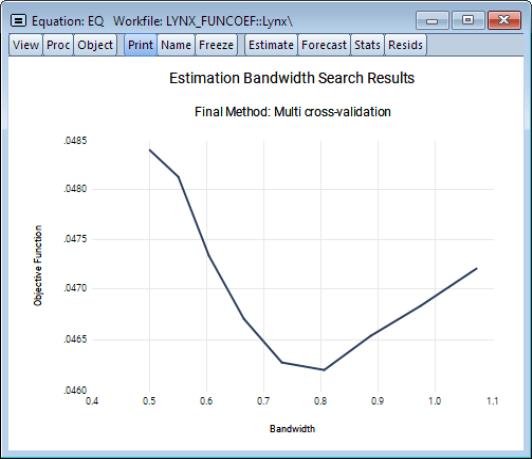
• New views permit examination of the bandwidth selection procedure results for both pilot and final bandwidths, and functional bias curves.
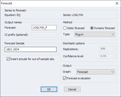
• Sophisticated forecasting engine performs static and dynamic forecasting via plug-in, Monte Carlo (asymptotic), Monte Carlo bootstrap, and full bootstrap methods. Stochastic resampling routines support computation of simulation based forecast standard errors and confidence intervals:
• New proc allows you to specify a local pilot bandwidth that is independent of the estimation pilot bandwidth for computation of diagnostic views.
Note that to support these new features, functional coefficients models estimated by EViews 12 are not backward compatible with earlier versions of EViews.
• In addition, there are a number of different views and procedures of interest that are new or enhanced. See
“Equations”.
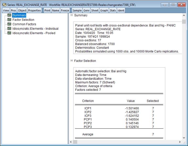
Cross-Sectionally Dependent Panel Unit Root Tests
Since many economic time series have short samples but are observed over many cross-sections, multivariate unit root tests that combine results for different cross-sections, colloquially referred to as first generation panel unit root tests, offered improved statistical power over their univariate counterparts. These first generation panel unit root tests involve unit root testing on pooled panel data, with (possibly) individual trend, intercepts, and lag coefficients. While this framework is a natural first step, it comes at the steep cost of requiring cross-sectional independence.
Tests which account for cross-sectional dependence have been termed second generation panel unit root tests. EViews current supports two important second generation contributions: Panel Analysis of Nonstationarity in Idiosyncratic and Common Components (PANIC) due to Bai and Ng (2004), and Cross-sectionally Augmented IPS (CIPS), developed by Pesaran (2007).
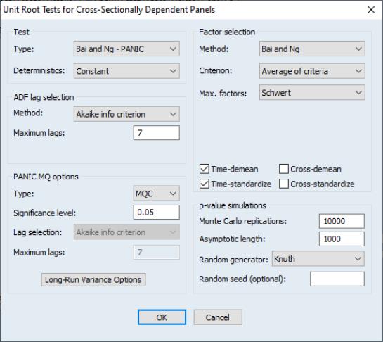
Second generation panel unit root tests may be performed on a single series in a panel workfile or on a group of series in a workfile. To perform the test in the panel setting, you should open the series and then click on EViews will display the dialog:
You may use the dropdown to choose PANIC or CIPS testing. Options include the lag selection for the ADF test, MQ testing, factor selection, and p-value simulation settings.
Note that in the group setting, you may perform the same test by opening the group object and clicking on .
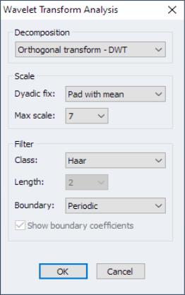
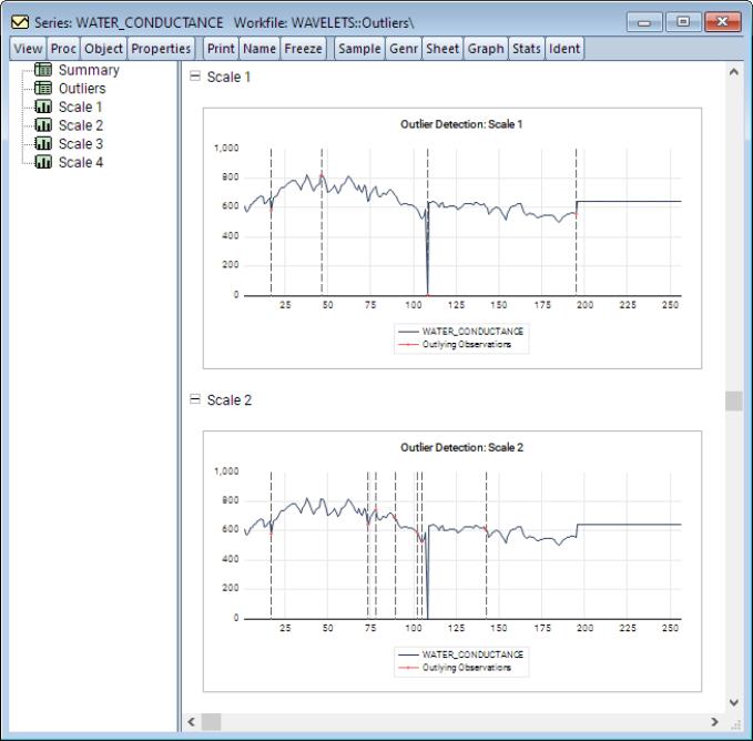
Wavelet Decomposition
Wavelet decomposition can decompose a series into its long-run behavior (smooths) and short run behavior (details). Among other things, wavelets may be used to
• compute the discrete wavelet transform to decompose a series into short and long run components at different scales
• obtain a long-run approximation to a series by neglecting transient features (thresholding)
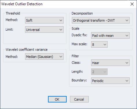
• detect outliers
• decompose a series variance
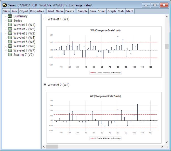
EViews offers an easy to use interface for each of these tasks. For example, To perform wavelet decomposition in EViews 12, open the series of interest and select
There are several entries under this menu item, each with its own set of options. The spool output lets you examine many features of the decomposition:
To detect outliers, select
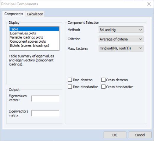
Number of Factor Selection Methods
EViews 12 adds the Bain and Ng (200) and Ahn and Horenstein (2013) methods for determining the number of factors to retain to our existing principal components and factor analysis engines.
• See
“Factor”for estimation methods and factor views that use the new factor selection methods.