Pool
Pooled time series, cross-section object. Used when working with data with both time series and cross-section structure.
Pool Declaration
pool declare pool object.
To declare a pool object, use the pool keyword, followed by a pool name, and optionally, a list of pool members. Pool members are short text identifiers for the cross section units:
pool mypool
pool g7 _can _fr _ger _ita _jpn _us _uk
Pool Methods
ls estimate linear regression models including cross-section weighted least squares, and fixed and random effects models.
tsls linear two-stage least squares (TSLS) regression models.
Pool Views
cellipse Confidence ellipses for coefficient restrictions.
coefcov coefficient covariance matrix.
coint Johansen’s cointegration test.
describe calculate pool descriptive statistics.
fixedtest test significance of estimates of fixed effects.
label label information for the pool object.
output table of estimation results.
ranhaus Hausman test for correlation between random effects and regressors.
resids table or graph of residuals for each pool member.
results table of estimation results.
sheet spreadsheet view of series in pool.
testadd likelihood ratio test for adding variables to pool equation.
testdrop likelihood ratio test for dropping variables from pool equation.
uroot unit root test on a pool series.
uroot2 dependent (second generation panel) unit root tests on a pool series .
wald Wald coefficient restriction test.
Pool Procs
add add cross section members to pool.
clearhist clear the contents of the history attribute.
copy creates a copy of the pool.
define define cross section identifiers.
drop drop cross section members from pool.
fetch fetch series into workfile using a pool.
genr generate pool series using the “?”.
makegroup create a group of series from a pool.
makemodel creates a model object from the estimated pool.
makeresids make series containing residuals from pool.
makesystem creates a system object from the pool for other estimation methods.
olepush push updates to OLE linked objects in open applications.
read import pool data from disk.
setattr set the value of an object attribute.
store store pool series in database/bank files.
write export pool data to disk.
Pool Data Members
String Values
@attr("arg") string containing the value of the arg attribute, where the argument is specified as a quoted string.
@command full command line form of the estimation command. Note this is a combination of @method, @options and @spec.
@crossids space delimited list of the Pool identifiers.
@crossidsest space delimited list of the Pool identifiers used in estimation.
@description string containing the Pool object’s description (if available).
@detailedtype returns a string with the object type: “POOL”.
@displayname returns the Pool’s display name. If the Pool has no display name set, the name is returned.
@idname(i) i-th cross-section identifier.
@idnameest(i) i-th cross-section identifier for estimated equation.
@method command line form of estimation method (“LS”, “TSLS”, etc....).
@name returns the Pool’s name.
@options command line form of pool estimation options.
@remarks string containing the pool object’s remarks (if available).
@smpl description of sample used for estimation.
@spec original Pool estimation specification.
@type returns a string with the object type: “POOL”.
@updatetime returns a string representation of the time and date at which the Pool was last updated.
Scalar Values
@aic Akaike information criterion.
@coefcov(i,j) covariance of coefficients i and j.
@coefs(i) coefficient i.
@dw Durbin-Watson statistic.
@effects(i) estimated fixed or random effect for the i-th cross-section member (only for fixed or random effects).
@f F-statistic.
@logl log likelihood.
@meandep mean of the dependent variable.
@ncoef total number of estimated coefficients.
@ncross total number of cross sectional units.
@ncrossest number of cross sectional units in last estimated pool equation.
@npers number of workfile periods used in estimation of the pool equation.
@r2 R-squared statistic.
@rbar2 adjusted R-squared statistic.
@regobs total number of observations in regression.
@schwarz Schwarz information criterion.
@sddep standard deviation of the dependent variable.
@se standard error of the regression.
@ssr sum of squared residuals.
@stderrs(i) standard error for coefficient i.
@totalobs total number of observations in the pool. For a balanced sample this is “@regobs*@ncrossest”.
@tstats(i) t-statistic value for coefficient i.
c(i) i-th element of default coefficient vector for the pool.
Vectors and Matrices
@coefcov covariance matrix for coefficients of equation.
@coefs coefficient vector.
@effects vector of estimated fixed or random effects (only for fixed or random effects estimation).
@residcov (sym) covariance matrix of the residuals.
@stderrs vector of standard errors for coefficients.
@tstats vector of t-statistic values for coefficients.
Pool Examples
To read data using the pool object:
mypool1.read(b2) data.xls x? y? z?
To delete and store pool series you may enter:
mypool1.delete x? y?
mypool1.store z?
Descriptive statistics may be computed using the command:
mypool1.describe(m) z?
To estimate a pool equation using least squares and to access the t-statistics, enter:
mypool1.ls y? c z? @ w?
vector tstat1 = mypool1.@tstats
Add cross section members to a pool.
Syntax
pool_name.add id1 [id2 id3 ...]
List the cross-section identifiers to add to the pool.
Examples
countries.add us gr
Adds US and GR as cross-section members of the pool object COUNTRIES.
Cross-references
See
“Cross-section Identifiers” for a discussion of pool identifiers.
Confidence ellipses for coefficient restrictions.
The cellipse view displays confidence ellipses for pairs of coefficient restrictions for an estimation from a pool object.
Syntax
pool_name.cellipse(options) restrictions
Enter the object name, followed by a period, and the keyword cellipse. This should be followed by a list of the coefficient restrictions. Joint (multiple) coefficient restrictions should be separated by commas.
Options
ind=arg | Specifies whether and how to draw the individual coefficient intervals. The default is “ind=line” which plots the individual coefficient intervals as dashed lines. “ind=none” does not plot the individual intervals, while “ind=shade” plots the individual intervals as a shaded rectangle. |
size= number (default=0.95) | Set the size (level) of the confidence ellipse. You may specify more than one size by specifying a space separated list enclosed in double quotes. |
dist= arg | Select the distribution to use for the critical value associated with the ellipse size. The default depends on estimation object and method. If the parameter estimates are least-squares based, the  distribution is used; if the parameter estimates are likelihood based, the  distribution will be employed. “dist=f” forces use of the F-distribution, while “dist=c” uses the  distribution. |
prompt | Force the dialog to appear from within a program. |
p | Print the graph. |
Examples
The two commands:
pool1.cellipse c(1), c(2), c(3)
pool1.cellipse c(1)=0, c(2)=0, c(3)=0
both display a graph showing the 0.95-confidence ellipse for C(1) and C(2), C(1) and C(3), and C(2) and C(3).
pool1.cellipse(dist=c,size="0.9 0.7 0.5") c(1), c(2)
displays multiple confidence ellipses (contours) for C(1) and C(2).
Cross-references
Clear the contents of the history attribute for pool objects.
Removes the pool’s history attribute, as shown in the label view of the pool.
Syntax
pool_name.clearhist
Examples
p1.clearhist
p1.label
The first line removes the history from the pool P1, and the second line displays the label view of P1, including the now blank history field.
Cross-references
See
“Labeling Objects” for a discussion of labels and display names.
Clear the contents of the remarks attribute.
Removes the pool’s remarks attribute, as shown in the label view of the pool.
Syntax
pool_name.clearremarks
Examples
p1.clearremarks
p1.label
The first line removes the remarks from the pool P1, and the second line displays the label view of P1, including the now blank remarks field.
Cross-references
See
“Labeling Objects” for a discussion of labels and display names.
Coefficient covariance matrix.
Displays the covariances of the coefficient estimates for an estimated pool object.
Syntax
pool_name.coefcov(options)
Options
p | Print the coefficient covariance matrix. |
Examples
pool1.coefcov
displays the coefficient covariance matrix for POOL1 in a window. To store the coefficient covariance matrix as a sym object, use “@coefcov”:
sym eqcov = pool1.@coefcov
Cross-references
Panel cointegration tests.
Syntax
pool_name.coint(option) pool_ser1 pool_ser2 [pool_ser3]...
Follow the pool name with the coint keyword, any options, and a list of two or more ordinary or pool series.
Options
You may specify the type using one of the following keywords:
Pedroni (default) | Pedroni (1994 and 2004). |
Kao | Kao (1999) |
Fisher | Fisher - pooled Johansen |
Depending on the type selected above, the following may be used to indicate deterministic trends:
const (default) | Include a constant in the test equation. Applicable to Pedroni and Kao tests. |
trend | Include a constant and a linear time trend in the test equation. Applicable to Pedroni tests. |
none | Do not include a constant or time trend. Applicable to Pedroni tests. |
a | No deterministic trend in the data, and no intercept or trend in the cointegrating equation. Applicable to Fisher tests. |
b | No deterministic trend in the data, and an intercept but no trend in the cointegrating equation. Applicable to Fisher tests. |
c | Linear trend in the data, and an intercept but no trend in the cointegrating equation. Applicable to Fisher tests. |
d | Linear trend in the data, and both an intercept and a trend in the cointegrating equation. Applicable to Fisher tests. |
e | Quadratic trend in the data, and both an intercept and a trend in the cointegrating equation. Applicable to Fisher tests. |
Additional options:
ac=arg (default= “bt”) | Method of estimating the frequency zero spectrum: “bt” (Bartlett kernel), “pr” (Parzen kernel), “qs” (Quadratic Spectral kernel). Applicable to Pedroni and Kao tests. |
band=arg (default= “nw”) | Method of selecting the bandwidth, where arg may be “nw” (Newey-West automatic variable bandwidth selection), or a number indicating a user-specified common bandwidth. Applicable to Pedroni and Kao tests. |
lag=arg | For Pedroni and Kao tests, the method of selecting lag length (number of first difference terms) to be included in the residual regression. For Fisher tests, a pair of numbers indicating lag. |
info=arg (default= “sic”) | Information criterion to use when computing automatic lag length selection: “aic” (Akaike), “sic” (Schwarz), “hqc” (Hannan-Quinn). Applicable to Pedroni and Kao tests. |
maxlag=int | Maximum lag length to consider when performing automatic lag length selection, where int is an integer. The default= 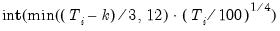 where  is the length of the cross-section. Applicable to Pedroni and Kao tests. |
disp=arg (default=500) | Maximum number of individual results to be displayed. |
prompt | Force the dialog to appear from within a program. |
p | Print results. |
Examples
pool01.coint(fisher,lag=1 2,c) y? x1? x2?
performs a Johansen test for pool series Y?, X1?, and X2? with a lag of 1 to 2 and linear trend in the data, and an intercept but no trend in the cointegrating equation is assumed as exogenous variables.
Cross-references
See
“References” for details on panel cointegration testing. See also
Pool::uroot.
Creates a copy of the pool.
Creates either a named or unnamed copy of the pool.
Syntax
pool_name.copy
pool_name.copy dest_name
Examples
p1.copy
creates an unnamed copy of the pool P1.
p1.copy p2
creates P2, a copy of the pool P1.
Cross-references
Define cross section members (identifiers) in a pool.
Syntax
pool_name.define id1 [id2 id3 ...]
List the cross section identifiers after the define keyword.
Examples
pool spot uk jpn ger can
spot.def uk ger ita fra
The first line declares a pool object named SPOT with cross section identifiers UK, JPN, GER, and CAN. The second line redefines the identifiers to be UK, GER, ITA, and FRA.
Cross-references
See
“Pooled Time Series, Cross-Section Data” for a discussion of cross-section identifiers.
Deletes series based upon identifiers in a pool.
Syntax
pool_name.delete(option) pool_ser1 [pool_ser2 pool_ser3 ...]
Follow the keyword by a list of the names of any series you wish to remove from the current workfile. Deleting does not remove objects that have been stored on disk in EViews database files.
The delete command allows you to delete series from the workfile using ordinary and pool series names.
You can delete an object from a database by prefixing the name with the database name and a double colon. You can use a pattern to delete all objects from a workfile or database with names that match the pattern. Use the “?” to match any one character and the “*” to match zero or more characters.
If you use delete in a program file, EViews will delete the listed objects without prompting you to confirm each deletion.
Options
prompt | Force the dialog to appear from within a program. |
Examples
To delete all series in the workfile with names beginning with “CPI” that are followed by identifiers in the pool object MYPOOL:
mypool.delete cpi?
Cross-references
See
“Object Basics” for a discussion of working with objects, and
“EViews Databases” for a discussion of EViews databases.
Computes and displays descriptive statistics for the pooled data.
Syntax
pool_name.describe(options) pool_ser1 [pool_ser2 pool_ser3 ...]
List the name of ordinary and pool series for which you wish to compute descriptive statistics.
By default, statistics are computed for each stacked pool series, using only common observations where all of the cross-sections for a given series have nonmissing data. A missing observation for a series in any one cross-section causes that observation to be dropped for all cross-sections for the corresponding series. You may change the default treatment of NAs using the “i” and “b” options.
EViews also allows you to compute statistics with the cross-section means removed, statistics for each cross-sectional series in a pool series, and statistics for each period, taken across all cross-section units.
Options
m | Stack data and subtract cross-section specific means from each variable—this option provides the within estimators. |
c | Do not stack data—compute statistics individually for each cross-sectional unit. |
t | Time period specific—compute statistics for each period, taken over all cross-section identifiers. |
i | Individual sample—includes every valid observation for the series even if data are missing from other series in the list. |
b | Balanced sample—constrains each cross-section to have the same observations. If an observation is missing for any series, in any cross-section, it will be dropped for all cross-sections. |
prompt | If no pool series are specified, force the dialog to appear from within a program. |
p | Print the descriptive statistics. |
Examples
pool1.describe(m) gdp? inv? cpi?
displays the “within” descriptive statistics of the three series GDP, INV, CPI for the POOL1 cross-section members.
pool1.describe(t) gdp?
computes the statistics for GDP for each period, taken across each of the cross-section identifiers.
Cross-references
See
“Pooled Time Series, Cross-Section Data” for a discussion of the computation of these statistics, and a description of individual and balanced samples.
Display table, graph, or spool output in the pool object window.
Display the contents of a table, graph, or spool in the window of the pool object.
Syntax
pool_name.display object_name
Examples
pool1.display tab1
Display the contents of the table TAB1 in the window of the object POOL1.
Cross-references
Most often used in constructing an EViews Add-in. See
“Custom Object Output”.
Display name for pool objects.
Attaches a display name to a pool object which may be used to label output in place of the standard pool object name.
Syntax
pool_name.displayname display_name
Display names are case-sensitive, and may contain a variety of characters, such as spaces, that are not allowed in pool object names.
Examples
hrs.displayname Hours Worked
hrs.label
The first line attaches a display name “Hours Worked” to the pool object HRS, and the second line displays the label view of HRS, including its display name.
Cross-references
See
“Labeling Objects” for a discussion of labels and display names.
Drops cross-section members from a pool.
Syntax
pool_name.drop id1 [id2 id3 ...]
List the cross-section members to be dropped from the pool.
Examples
crossc.drop jpn kor hk
drops the cross-section members JPN, KOR, and HK from the pool CROSSSC.
Cross-references
“Cross-section Identifiers” discusses pool identifiers.
Fetch objects from databases or databank files into the workfile.
fetch reads one or more objects from EViews databases or databank files into the active workfile. The objects are loaded into the workfile using the object in the database or using the databank file name. EViews will first expand the list of series using the pool operator, and then perform the fetch.
If you fetch a series into a workfile with a different frequency, EViews will automatically apply the frequency conversion method attached to the series by setconvert. If the series does not have an attached conversion method, EViews will use the method set by in the main menu. You can override the conversion method by specifying an explicit conversion method option.
Syntax
pool_name.fetch(options) pool_ser1 [pool_ser2 pool_ser3 ...]
The fetch command keyword is followed by a list of object names separated by spaces. The default behavior is to fetch the objects from the default database (this is a change from versions of EViews prior to EViews 3.x where the default was to fetch from individual databank files).
You can precede the object name with a database name and the double colon “::” to indicate a specific database source. If you specify the database name as an option in parentheses (see below), all objects without an explicit database prefix will be fetched from the specified database. You may optionally fetch from individual databank files or search among registered databases.
You may use wild card characters, “?” (to match a single character) or “*” (to match zero or more characters), in the object name list. All objects with names matching the pattern will be fetched.
To fetch from individual databank files that are not in the default path, you should include an explicit path. If you have more than one object with the same file name (for example, an equation and a series named CONS), then you should supply the full object file name including identifying extensions.
Options
d=db_name | Fetch from specified database. |
d | Fetch all registered databases in registry order. |
i | Fetch from individual databank files. |
notifyillegal | When in a program, report illegal EViews object names. By default, objects with illegal names are automatically renamed. (Has no effect in the command window.) |
prompt | Force the dialog to appear from within a program. |
The database specified by the double colon “::” takes precedence over the database specified by the “d=” option.
In addition, there are a number of options for controlling automatic frequency conversion when performing a fetch. The following options control the frequency conversion method when copying series and group objects to a workfile, converting from low to high frequency:
c=arg | Low to high conversion methods: “r” (constant match average), “d” (constant match sum), “q” (quadratic match average), “t” (quadratic match sum), “i” (linear match last), “c” (cubic match last). |
The following options control the frequency conversion method when copying series and group objects to a workfile, converting from high to low frequency:
c=arg | High to low conversion methods removing NAs: “a” (average of the nonmissing observations), “s” (sum of the nonmissing observations), “f” (first nonmissing observation), “l” (last nonmissing observation), “x” (maximum nonmissing observation), “m” (minimum nonmissing observation). High to low conversion methods propagating NAs: “an” or “na” (average, propagating missings), “sn” or “ns” (sum, propagating missings), “fn” or “nf” (first, propagating missings), “ln” or “nl” (last, propagating missings), “xn” or “nx” (maximum, propagating missings), “mn” or “nm” (minimum, propagating missings). |
If no conversion method is specified, the series-specific or global default conversion method will be employed.
Examples
To fetch M1, GDP, and UNEMP pool series from the default database, use:
pool1.fetch m1? gdp? unemp?
To fetch M1 and GDP from the US1 database and UNEMP from the MACRO database, use the command:
pool1.fetch(d=us1) m1? gdp? macro::unemp
Use the “notifyillegal” option to display a dialog when fetching the series MYILLEG@LNAME that will suggest a valid name and give you to opportunity to name the object before it is inserted into a workfile:
pool2.fetch(notifyillegal) myilleg@lname
Cross-references
See
“EViews Databases” for a discussion of databases, databank files, and frequency conversion.
Appendix A. “Wildcards” describes the use of wildcard characters.
Test joint significance of the fixed effects estimates.
Tests the hypothesis that the estimated fixed effects are jointly significant using

and LR test statistics. If the estimated specification involves two-way fixed effects, three separate tests will be performed; one for each set of effects, and one for the joint effects.
Only valid for panel or pool regression equations estimated with fixed effects. Not currently available for specifications estimated using instrumental variables.
Syntax
pool_name.fixedtest(options)
Options
p | Print output from the test. |
Examples
pool1.fixedtest
tests whether the fixed effects are jointly significant.
Cross-references
Generate series.
This procedure allows you to generate multiple series using the cross-section identifiers in a pool.
Syntax
pool_name.genr(option) ser_name = expression
You may use the cross section identifier “?” in the series name and/or in the expression on the right-hand side.
Options
prompt | Force the dialog to appear from within a program. |
Examples
The commands,
pool pool1
pool1.add 1 2 3
pool1.genr y? = x? - @mean(x?)
are equivalent to generating separate series for each cross-section:
genr y1 = x1 - @mean(x1)
genr y2 = x2 - @mean(x2)
genr y3 = x3 - @mean(x3)
Similarly:
pool pool2
pool2.add us uk can
pool2.genr y_? = log(x_?) - log(x_us)
generates three series Y_US, Y_UK, Y_CAN that are the log differences from X_US. Note that Y_US=0.
It is worth noting that the pool genr command simply loops across the cross-section identifiers, performing the evaluations using the appropriate substitution. Thus, the command,
pool2.genr z = y_?
is equivalent to entering:
genr z = y_us
genr z = y_uk
genr z = y_can
so that upon completion, the ordinary series Z will contain Y_CAN.
Cross-references
See
“Pooled Time Series, Cross-Section Data” for a discussion of the computation of pools, and a description of individual and balanced samples.
See
Series::series for a discussion of the expressions allowed in
genr.
Display or change the label view of a pool object, including the last modified date and display name (if any).
As a procedure, label changes the fields in the pool object label.
Syntax
pool_name.label
pool_name.label(options) [text]
Options
The first version of the command displays the label view of the pool object. The second version may be used to modify the label. Specify one of the following options along with optional text. If there is no text provided, the specified field will be cleared.
c | Clears all text fields in the label. |
d | Sets the description field to text. |
s | Sets the source field to text. |
u | Sets the units field to text. |
r | Appends text to the remarks field as an additional line. |
p | Print the label view. |
Examples
The following lines replace the remarks field of POOL1 with “Data from CPS 1988 March File”:
pool1.label(r)
pool1.label(r) Data from CPS 1988 March File
To append additional remarks to POOL1, and then to print the label view:
pool1.label(r) Log of hourly wage
pool1.label(p)
To clear and then set the units field, use:
pool1.label(u) Millions of bushels
Cross-references
See
“Labeling Objects” for a discussion of labels.
Estimation by linear or nonlinear least squares regression.
ls estimates cross-section weighed least squares, feasible GLS, and fixed and random effects models.
Syntax
pool_name.ls(options) y [x1 x2 x3...] [@cxreg z1 z2 ...] [@perreg z3 z4 ...]
ls carries out pooled data estimation. Type the name of the dependent variable followed by one or more lists of regressors. The first list should contain ordinary and pool series that are restricted to have the same coefficient across all members of the pool. The second list, if provided, should contain pool variables that have different coefficients for each cross-section member of the pool. If there is a cross-section specific regressor list, the two lists must be separated by “@CXREG”. The third list, if provided, should contain pool variables that have different coefficients for each period. The list should be separated from the previous lists by “@PERREG”.
You may include AR terms as regressors in either the common or cross-section specific lists. AR terms are, however, not allowed for some estimation methods. MA terms are not supported.
Options
m=integer | Set maximum number of iterations. |
c=scalar | Set convergence criterion. The criterion is based upon the maximum of the percentage changes in the scaled coefficients. The criterion will be set to the nearest value between 1e-24 and 0.2. |
s | Use the current coefficient values in “C” as starting values for equations with AR or MA terms (see also
param). |
s=number | Determine starting values for equations specified by list with AR or MA terms. Specify a number between zero and one representing the fraction of preliminary least squares estimates computed without AR or MA terms to be used. Note that out of range values are set to “s=1”. Specifying “s=0” initializes coefficients to zero. By default EViews uses “s=1”. |
numericderiv / ‑numericderiv | [Do / do not] use numeric derivatives only. If omitted, EViews will follow the global default. |
fastderiv / ‑fastderiv | [Do / do not] use fast derivative computation. If omitted, EViews will follow the global default. |
showopts / ‑showopts | [Do / do not] display the starting coefficient values and estimation options in the estimation output. |
cx=arg | Cross-section effects: (default) none, fixed effects (“cx=f”), random effects (“cx=r”). |
per=arg | Period effects: (default) none, fixed effects (“per=f”), random effects (“per=r”). |
wgt=arg | GLS weighting: (default) none, cross-section system weights (“wgt=cxsur”), period system weights (“wgt=persur”), cross-section diagonal weighs (“wgt=cxdiag”), period diagonal weights (“wgt=perdiag”). |
cov=arg | Coefficient covariance method: (default) ordinary, White cross-section system (period clustering) robust (“cov=cxwhite” or “cov=percluster”), White period system (cross-section clustering) robust (“cov=perwhite” or “cov=cxcluster”), White heteroskedasticity robust (“cov=stackedwhite”), White two-way cluster robust (cov=bothcluster”), Cross-section system robust/PCSE (“cov=cxsur”), Period system robust/PCSE (“cov=persur”), Cross-section heteroskedasticity robust/PCSE (“cov=cxdiag”), Period heteroskedasticity robust/PCSE (“cov=perdiag”). |
keepwgts | Keep full set of GLS weights used in estimation with object, if applicable (by default, only small memory weights are saved). |
rancalc=arg (default=“sa”) | Random component method: Swamy-Arora (“rancalc=sa”), Wansbeek-Kapteyn (“rancalc=wk”), Wallace-Hussain (“rancalc=wh”). |
nodf | Do not perform degree of freedom corrections in computing coefficient covariance matrix. The default is to use degree of freedom corrections. |
b | Estimate using a balanced sample (pool estimation only). |
coef=arg | Specify the name of the coefficient vector (if specified by list); the default behavior is to use the “C” coefficient vector. |
iter=arg (default= “onec”) | Iteration control for GLS specifications: perform one weight iteration, then iterate coefficients to convergence (“iter=onec”), iterate weights and coefficients simultaneously to convergence (“iter=sim”), iterate weights and coefficients sequentially to convergence (“iter=seq”), perform one weight iteration, then one coefficient step (“iter=oneb”). Note that random effects models currently do not permit weight iteration to convergence. |
unbalsur | Compute SUR factorization for unbalanced data using the subset of available observations in a cluster. |
prompt | Force the dialog to appear from within a program. |
p | Print basic estimation results. |
Examples
pool1.ls dy? c inv? edu? year
estimates pooled OLS of DY? on a constant, INV?, EDU? and YEAR.
pool1.ls(cx=f) dy? @cxreg inv? edu? year ar(1)
estimates a fixed effects model without restricting any of the coefficients to be the same across pool members.
Cross-references
“Basic Regression Analysis” and
“Additional Regression Tools” discuss the various regression methods in greater depth.
See
“Pooled Time Series, Cross-Section Data” for a discussion of pool estimation, and
“Panel Estimation” for a discussion of panel equation estimation.
See
“Special Expression Reference” for special terms that may be used in
ls specifications.
See also
Pool::tsls for instrumental variables estimation.
Make a group out of pool and ordinary series using a pool object.
Syntax
pool_name.makegroup(group_name, options) pool_series1 [pool_series2 pool_series3…]
List the ordinary and pool series to be placed in the group. If specified, group_name should be the first option.
Options
prompt | Force the dialog to appear from within a program. |
Examples
pool1.makegroup(g1) x? z y?
places the ordinary series Z, and all of the series represented by the pool series X? and Y?, in the group G1.
Cross-references
Make a model from a pool object.
Syntax
pool_name.makemodel(name) assign_statement
If you provide a name for the model in parentheses after the keyword, EViews will create the named model in the workfile. If you do not provide a name, EViews will open an untitled model window if the command is executed from the command line.
Examples
pool3.ls m1? gdp? tb3?
pool3.makemodel(poolmod) @prefix s_
estimates a VAR and makes a model named POOLMOD from the estimated pool object. POOLMOD includes an assignment statement “ASSIGN @PREFIX S_”. Use the command “show poolmod” or “poolmod.spec” to open the POOLMOD window.
Cross-references
See
“Models” for a discussion of specifying and solving models in EViews.
Create residual series.
Creates and saves residuals in the workfile from a pool object.
Syntax
pool_name.makeresids [poolser]
Follow the object name with a period and the makeresids keyword, then provide a list of names to be given to the stored residuals. You may use a cross section identifier “?” to specify a set of names.
Options
n=arg | Create group object to hold the residual series. |
Examples
pool1.makeresids res1_?
The residuals of each pool member will have a name starting with “RES1_” and the cross-section identifier substituted for the “?”.
Cross-references
Create and save series of descriptive statistics computed from a pool object.
Syntax
pool_name.makestats(options) pool_series1 [pool_series2 ...] @ stat_list
You should provide options, a list of series names, an “@” separator, and a list of command names for the statistics you wish to compute. The series will have a name with the cross-section identifier “?” replaced by the statistic command.
Options
Options in parentheses specify the sample to use to compute the statistics
i | Use individual sample. |
c (default) | Use common sample. |
b | Use balanced sample. |
o | Force the overwrite of the computed statistics series if they already exist. The default creates a new series using the next available names. |
prompt | Force the dialog to appear from within a program. |
Command names for the statistics to be computed
obs | Number of observations. |
mean | Mean. |
med | Median. |
var | Variance. |
sd | Standard deviation. |
skew | Skewness. |
kurt | Kurtosis. |
jarq | Jarque-Bera test statistic. |
min | Minimum value. |
max | Maximum value. |
Examples
pool1.makestats gdp_? edu_? @ mean sd
computes the mean and standard deviation of the GDP_? and EDU_? series in each period (across the cross-section members) using the default common sample. The mean and standard deviation series will be named GDP_MEAN, EDU_MEAN, GDP_SD, and EDU_SD.
pool1.makestats(b) gdp_? @ max min
Computes the maximum and minimum values of the GDP_? series in each period using the balanced sample. The max and min series will be named GDP_MAX and GDP_MIN.
Cross-references
See
“Pooled Time Series, Cross-Section Data” for details on the computation of these statistics and a discussion of the use of individual, common, and balanced samples in pool.
Create system from a pool object.
Syntax
pool_name.makesystem(options) y [x1 x2 x3 ...] [@cxeg w1 w2 ...] [@inst z1 z2 ...] [@cxinst z3 z4 ...]
Creates a system out of the pool equation specification. Each cross-section in the pool will be used to form an equation. The pool variable y is the dependent variable. The [x1 x2 x3 ...] list consists of regressors with common coefficients in the system. The @cxreg list are regressors with different coefficients in each cross-section. The list of variables that follow @inst are the common instruments. The list of variables that follow @cxinst are the equation specific instruments.
Note that period specific coefficients and effects are not available in this routine.
Options
name=name | Specify name for the system object. |
prompt | Force the dialog to appear from within a program. |
Examples
pool1.makesystem(name=sys1) inv? cap? @inst val?
creates a system named SYS1 with INV? as the dependent variable and a common intercept for each cross-section member. The regressor CAP? is restricted to have the same coefficient in each equation, while the VAL? regressor has a different coefficient in each equation.
pool1.makesystem(name=sys2,cx=f) inv? @cxreg cap? @cxinst @trend inv?(-1)
This command creates a system named SYS2 with INV? as the dependent variable and a different intercept for each cross-section member equation. The regressor CAP? enters each equation with a different coefficient and each equation has two instrumental variables @TREND and INV? lagged.
Cross-references
See
“System Estimation” for a discussion of system objects in EViews.
Push updates to OLE linked objects in open applications.
Syntax
pool_name.olepush
Cross-references
See
“Object Linking and Embedding (OLE)” for a discussion of using OLE with EViews.
Display estimation output.
output changes the default object view to display the estimation output (equivalent to using
Pool::results).
Syntax
pool_name.output
Options
p | Print estimation output for estimation object |
Examples
The output keyword may be used to change the default view of an estimation object. Entering the command:
pool1.output
displays the estimation output for pool POOL1.
Cross-references
Declare pool object.
Syntax
pool name [id1 id2 id3 …]
Follow the
pool keyword with a
name for the pool object. You may optionally provide the identifiers for the cross-section members of the pool object. Pool identifiers may be added or removed at any time using
Pool::add and
Pool::drop.
Examples
pool zoo1 dog cat pig owl ant
Declares a pool object named ZOO1 with the listed cross-section identifiers.
Cross-references
See
“Pooled Time Series, Cross-Section Data” for a discussion of working with pools in EViews.
See
Pool::add and
Pool::drop. See also
Pool::ls for details on estimation using a pool object.
Test for correlation between random effects and regressors using Hausman test.
Tests the hypothesis that the random effects (components) are correlated with the right-hand side variables in a pool equation setting. Uses Hausman test methodology to compare the results from the estimated random effects specification and a corresponding fixed effects specification. If the estimated specification involves two-way random effects, three separate tests will be performed; one for each set of effects, and one for the joint effects.
Only valid for pool regression equations estimated with random effects. Note that the test results may be suspect in cases where robust standard errors are employed.
Syntax
pool_name.ranhaus(options)
Options
p | Print output from the test. |
Examples
poo11.ls(cx=r) sales? c adver? lsales?
pool1.ranhaus
estimates a specification with cross-section random effects and tests whether the random effects are correlated with the right-hand side variables ADVER and LSALES using the Hausman test methodology.
Cross-references
Import data from a foreign disk file into a pool object.
May be used to import data into an existing workfile from a text, Excel, or Lotus file on disk.
Syntax
pool_name.read(options) [path\]file_name pool_ser1 [pool_ser2 pool_ser3 ...]
You must supply the name of the source file. If you do not include the optional path specification, EViews will look for the file in the default directory. Path specifications may point to local or network drives. If the path specification contains a space, you may enclose the entire expression in double quotation marks.
Follow the source file name with a list of ordinary or pool series.
Options
prompt | Force the dialog to appear from within a program. |
File type options
t=dat, txt | ASCII (plain text) files. |
t=wk1, wk3 | Lotus spreadsheet files. |
t=xls | Excel spreadsheet files. |
If you do not specify the “t” option, EViews uses the file name extension to determine the file type. If you specify the “t” option, the file name extension will not be used to determine the file type.
Options for ASCII text files
t | Read data organized by series. Default is to read by observation with series in columns. |
na=text | Specify text for NAs. Default is “NA”. |
d=t | Treat tab as delimiter (note: you may specify multiple delimiter options). The default is “d=c” only. |
d=c | Treat comma as delimiter. |
d=s | Treat space as delimiter. |
d=a | Treat alpha numeric characters as delimiter. |
custom = symbol | Specify symbol/character to treat as delimiter. |
mult | Treat multiple delimiters as one. |
names | Series names provided in file. |
label=integer | Number of lines between the header line and the data. Must be used with the “name” option. |
rect (default) / norect | [Treat / Do not treat] file layout as rectangular. |
skipcol = integer | Number of columns to skip. Must be used with the “rect” option. |
skiprow = integer | Number of rows to skip. Must be used with the “rect” option. |
comment= symbol | Specify character/symbol to treat as comment sign. Everything to the right of the comment sign is ignored. Must be used with the “rect” option. |
singlequote | Strings are in single quotes, not double quotes. |
dropstrings | Do not treat strings as NA; simply drop them. |
negparen | Treat numbers in parentheses as negative numbers. |
allowcomma | Allow commas in numbers (note that using commas as a delimiter takes precedence over this option). |
currency= symbol | Specify symbol/character for currency data. |
Options for spreadsheet (Lotus, Excel) files
t | Read data organized by series. Default is to read by observation with series in columns. |
letter_number (default=“b2”) | Coordinate of the upper-left cell containing data. |
s=sheet_name | Sheet name for Excel 5–8 Workbooks. |
Options for pool reading
bycross (default) / byper | Structure of stacked pool data [cross-section / date or period] (only for pool read). |
Examples
pool1.read(t=dat,na=.) a:\mydat.raw year lwage? hrs?
reads stacked data from an ASCII file MYDAT.RAW in the A: drive. The data in the file are stacked by cross-section, the missing value NA is coded as a “.” (dot or period). We read one ordinary series YEAR, and three two pool series LWAGE? and HRS?.
pool1.read(a2,s=sheet3,byper) statepan.xls inc? educ? pop?
reads data from an Excel file STATEPAN in the default directory. The data are stacked by period in the sheet SHEET3 with the upper left data cell A2. We read three pool series INC? EDUC? and POP?.
Cross-references
See
“Creating a Workfile by Reading from a Foreign Data Source” and
“Importing Data” for a discussion and examples of importing data from external files.
“Working with Panel Data” describes panel data alternatives to working with pooled data.
Display text of specification for pool objects.
Syntax
pool_name.representation(options)
Options
p | Print the representation text. |
Examples
pool1.representations
displays the specifications of the estimation object POOL1.
Cross-references
See
“Estimating a Pool Equation” for a discussion of pool equations.
Residual correlation matrix.
Displays the correlations of the residuals from each pool cross-section equation.
Syntax
pool_name.residcor(options)
Options
p | Print the correlation matrix. |
Examples
pool1.residcor
displays the residual correlation matrix of POOL1.
Cross-references
Residual covariance matrix.
Displays the covariances of the residuals from each pool cross-section equation.
Syntax
pool_name.residcov(options)
Options
p | Print the covariance matrix. |
Examples
pool1.residcov
displays the residual covariance matrix of POOL1.
Cross-references
See
“Estimating a Pool Equation” for a discussion of pool equations.
Display residuals.
Display the actual, fitted values and residuals in either tabular or graphical form. resids displays multiple graphs, where each graph will contain the residuals for each cross-section in the pool.
Syntax
pool_name.resids(options)
Options
g (default) | Display graph(s) of residuals. |
p | Print the table/graph. |
Examples
pool1.ls m1? c inc? tb3?
pool1.resids
regresses M1 on a constant, INC, and TB3, and displays a table of actual, fitted, and residual series.
pool1.resids(g)
displays a graph of the actual, fitted, and residual series.
Cross-references
Cross-references
See
“Estimating a Pool Equation” for a discussion of pool equations.
Displays the results view of a pool object.
Syntax
pool_name.results(options)
Options
Examples
pool1.ls m1? c inc? tb3?
pool1.results(p)
estimates an equation using least squares, and displays and prints the results.
Cross-references
See
“Estimating a Pool Equation” for a discussion of pool equations.
Set the object attribute.
Syntax
pool_name.setattr(attr) attr_value
Sets the attribute attr to attr_value. Note that quoting the arguments may be required. Once added to an object, the attribute may be extracted using the @attr data member.
Examples
a.setattr(revised) never
String s = a.@attr("revised")
sets the “revised” attribute in the object A to the string “never”, and extracts the attribute into the string object S.
Cross-references
Spreadsheet view of a pool object.
Syntax
pool_name.sheet(options) pool_ser1 [pool_ser2 pool_ser3 ...]
The sheet view displays the spreadsheet view of the series in the pool. Follow the word sheet by a list of series to display; you may use the cross section identifier “?” in the series name.
Options
prompt | Force the dialog to appear from within a program. |
p | Print the spreadsheet view. |
Examples
pool1.sheet(p) x? y? z?
displays and prints the pool spreadsheet view of the series X?, Y?, and Z?.
Cross-references
Store objects in databases and databank files.
Stores one or more objects in the current workfile in EViews databases or individual databank files on disk. The objects are stored under the name that appears in the workfile. EViews will first expand the list of series using the pool operator, and then perform the operation.
Syntax
pool_name.store(options) pool_ser1 [pool_ser2 pool_ser3 ...]
Follow the store command keyword with a list of object names (each separated by a space) that you wish to store. The default is to store the objects in the default database. (This behavior is a change from EViews 2 and earlier where the default was to store objects in individual databank files).
You may precede the object name with a database name and the double colon “::” to indicate a specific database. You can also specify the database name as an option in parentheses, in which case all objects without an explicit database name will be stored in the specified database.
You may use the wild card character “*” to match zero or more characters in the object name list. All objects with names matching the pattern will be stored. You may not use “?” as a wildcard character, since this conflicts with the pool identifier.
You can optionally choose to store the listed objects in individual databank files. To store in files other than the default path, you should include a path designation before the object name.
Options
d=db_name | Store to the specified database. |
i | Store to individual databank files. |
1 / 2 | Store series in [single / double] precision to save space. |
o | Overwrite object in database (default is to merge data, where possible). |
g=arg | Group store from workfile to database: “s” (copy group definition and series as separate objects), “t” (copy group definition and series as one object), “d” (copy series only as separate objects), “l” (copy group definition only). |
prompt | Force the dialog to appear from within a program. |
If you do not specify the precision option (1 or 2), the global option setting will be used. See
“Database Storage Defaults”.
Examples
pool1.store m1? gdp? unemp?
stores the three pool objects M1, GDP, UNEMP in the default database.
pool1.store(d=us1) m1? gdp? macro::unemp?
Cross-references
“Basic Data Handling” discusses exporting data in other file formats. See
“EViews Databases” for a discussion of EViews databases and databank files.
For additional discussion of wildcards, see
Appendix A. “Wildcards”.
Test whether to add regressors to an estimated equation.
Tests the hypothesis that the listed variables were incorrectly omitted from an estimated equation (only available for equations estimated by list). The test displays some combination of Wald and LR test statistics, as well as the auxiliary regression.
Syntax
pool_name.testadd(options) [x1 x2 ...] [@cxreg z1 z2 ...] [@perreg z3 z4 ...]
List the names of the series to test for omission after the keyword.
Options
prompt | Force the dialog to appear from within a program. |
p | Print output from the test. |
Examples
pool1.testadd gdp? @cxreg inc?
tests the addition of the pool series GDP? to the common coefficients list and INC? to the cross-section specific coefficients list.
Cross-references
See
“Coefficient Diagnostics” for further discussion.
Test whether to drop regressors from a regression.
Tests the hypothesis that the listed variables were incorrectly included in the estimated equation (only available for equations estimated by list). The test displays some combination of

and LR test statistics, as well as the test regression.
Syntax
pool_name.testdrop(options) arg1 [arg2 arg3 ...]
List the names of the series to test for omission after the keyword.
Options
prompt | Force the dialog to appear from within a program. |
p | Print output from the test. |
Examples
pool1.testdrop(p) x?
drops X? from the existing pool specification and prints the results of the test.
Cross-references
See
“Coefficient Diagnostics” for further discussion of testing coefficients.
Two-stage least squares.
Syntax
pool_name.tsls(options) y [x1 x2 x3 ...] [@cxreg w1 w2 ...] [@perreg w3 w4 ...] [@inst z1 z2 ...] [@cxinst z3 z4 ...] [@perinst z5 z6 ...]
Type the name of the dependent variable followed by one or more lists of regressors. The first list should contain ordinary and pool series that are restricted to have the same coefficient across all members of the pool. The second list, if provided, should contain pool variables that have different coefficients for each cross-section member of the pool. If there is a cross-section specific regressor list, the two lists must be separated by “@CXREG”. The third list, if provided, should contain pool variables that have different coefficients for each period. The list should be separated from the previous lists by “@PERREG”.
You may include AR terms as regressors in either the common or cross-section specific lists. AR terms are, however, not allowed for some estimation methods. MA terms are not supported.
Instruments should be specified in one of three lists. The “@INST” list should contain instruments that are common across all cross-sections and periods. The “@CXINST” should contain instruments that differ across cross-sections, while the “@PERINST” list specifies instruments that differ across periods.
There must be at least as many instrumental variables as there are independent variables. All exogenous variables included in the regressor list should also be included in the corresponding instrument list. A constant is included in the common instrumental list if not explicitly specified.
Options
General options
m=integer | Set maximum number of iterations. |
c=number | Set convergence criterion. The criterion is based upon the maximum of the percentage changes in the scaled coefficients. The criterion will be set to the nearest value between 1e-24 and 0.2. |
numericderiv / ‑numericderiv | [Do / do not] use numeric derivatives only. If omitted, EViews will follow the global default. |
fastderiv / ‑fastderiv | [Do / do not] use fast derivative computation. If omitted, EViews will follow the global default. |
showopts / ‑showopts | [Do / do not] display the starting coefficient values and estimation options in the estimation output. |
s | Use the current coefficient values in “C” as starting values for equations with AR or MA terms (see also
param). |
s=number | Determine starting values for equations specified by list with AR or MA terms. Specify a number between zero and one representing the fraction of preliminary least squares estimates computed without AR or MA terms. Note that out of range values are set to “s=1”. Specifying “s=0” initializes coefficients to zero. By default, EViews uses “s=1”. |
cx=arg | Cross-section effects. For fixed effects estimation, use “cx=f”; for random effects estimation, use “cx=r”. |
per=arg | Period effects. For fixed effects estimation, use “cx=f”; for random effects estimation, use “cx=r”. |
wgt=arg | GLS weighting: (default) none, cross-section system weights (“wgt=cxsur”), period system weights (“wgt=persur”), cross-section diagonal weighs (“wgt=cxdiag”), period diagonal weights (“wgt=perdiag”). |
cov=arg | Coefficient covariance method: (default) ordinary, White cross-section system robust (“cov=cxwhite”), White period system robust (“cov=perwhite”), White heteroskedasticity robust (“cov=stackedwhite”), Cross-section system robust/PCSE (“cov=cxsur”), Period system robust/PCSE (“cov=persur”), Cross-section heteroskedasticity robust/PCSE (“cov=cxdiag”), Period heteroskedasticity robust (“cov=perdiag”). |
keepwgts | Keep full set of GLS weights used in estimation with object, if applicable (by default, only small memory weights are saved). |
rancalc=arg (default=“sa”) | Random component method: Swamy-Arora (“rancalc=sa”), Wansbeek-Kapteyn (“rancalc=wk”), Wallace-Hussain (“rancalc=wh”). |
nodf | Do not perform degree of freedom corrections in computing coefficient covariance matrix. The default is to use degree of freedom corrections. |
coef=arg | Specify the name of the coefficient vector (if specified by list); the default is to use the “C” coefficient vector. |
iter=arg (default=“onec”) | Iteration control for GLS specifications: perform one weight iteration, then iterate coefficients to convergence (“iter=onec”), iterate weights and coefficients simultaneously to convergence (“iter=sim”), iterate weights and coefficients sequentially to convergence (“iter=seq”), perform one weight iteration, then one coefficient step (“iter=oneb”). Note that random effects models currently do not permit weight iteration to convergence. |
s | Use the current coefficient values in “C” as starting values for equations with AR or MA terms (see also
param). |
s=number | Determine starting values for equations specified by list with AR terms. Specify a number between zero and one representing the fraction of preliminary least squares estimates computed without AR terms. Note that out of range values are set to “s=1”. Specifying “s=0” initializes coefficients to zero. By default, EViews uses “s=1”. |
unbalsur | Compute SUR factorization in unbalanced data using the subset of available observations for a cluster. |
prompt | Force the dialog to appear from within a program. |
p | Print estimation results. |
Examples
pool1.tsls y? c x? @inst z?
estimates TSLS on the pool specification using common instruments Z?
Cross-references
See
“Two-stage Least Squares” and
“Two-Stage Least Squares” for details on two-stage least squares estimation in single equations and systems, respectively.
“Instrumental Variables” discusses estimation using pool objects, while
“Instrumental Variables Estimation” discusses estimation in panel structured workfiles.
Update coefficient object values from pool object.
Copies coefficients from the pool into the appropriate coefficient vector.
Syntax
pool_name.updatecoef
Follow the name of the pool object by a period and the keyword updatecoef.
Examples
pool1.ls y? c x1? x2? x3?
pool2.ls z? c z1? z2? z3?
pool1.updatecoef
places the coefficients from pool1 in the default coefficient vector C.
Cross-references
Carries out unit root tests on a pool series.
When used with a pool series, the procedure will perform panel unit root testing. The panel unit root tests include Levin, Lin and Chu (LLC), Breitung, Im, Pesaran, and Shin (IPS), Fisher - ADF, Fisher - PP, and Hadri tests on levels, or first or second differences.
Note that simulation evidence suggests that in various settings (for example, small

), Hadri's panel unit root test experiences significant size distortion in the presence of autocorrelation when there is no unit root. In particular, the Hadri test appears to over-reject the null of stationarity, and may yield results that directly contradict those obtained using alternative test statistics (see Hlouskova and Wagner (2006) for discussion and details).
Syntax
pool_name.uroot(options) pool_series
Enter the pool object name followed by a period, the keyword, and the name of a pool “?” series.
Options
Basic Specification Options
You should specify the exogenous variables and order of dependent variable differencing in the test equation using the following options:
exog=arg (default=“const”) | Specification of exogenous trend variables in the test equation: “const” “trend” (include a constant and a linear time trend). |
dif=integer (default=0) | Order of differencing of the series prior to running the test. Valid values are {0, 1, 2}. |
You may use one of the following keywords to specify the test:
sum (default) | Summary of the first five panel unit root tests (where applicable). |
llc | Levin, Lin, and Chu. |
breit | Breitung. |
ips | Im, Pesaran, and Shin. |
adf | Fisher - ADF. |
pp | Fisher - PP. |
hadri | Hadri. |
Sample Option
balance | Use balanced (across cross-sections or series) data when performing test. |
Lag Difference Options
Specifies the number of lag difference terms to be included in the test equation. Applicable in “Summary”, LLC, Breitung, IPS, and Fisher-ADF tests. The default setting depends on whether you choose to balance the samples across cross-sections.
If you do not include the “balance” option, the default is to perform automatic lag selection using the Schwarz criteria (“lagmethod=sic”).
Alternately, if you include the “balance” option, the default setting is a common, observation-based fixed lag (“lag=default”) where:
 | (1.3) |
lagmethod=arg (default=“sic”) | Method for selecting lag lengths (number of first difference terms) to be included in the Dickey-Fuller test regressions: “aic” (Akaike), “sic” (Schwarz), “hqc” (Hannan-Quinn), “tstat” (Ng-Perron first backward significant t-statistic). |
lag=arg | Specified lag length (number of first difference terms) to be included in the regression: integer (user-specified common lag length), vector_name (user-specific individual lag length, one row per cross-section). |
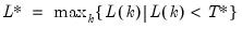
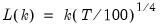
maxlag=arg | Maximum lag length to consider when performing automatic lag length selection: integer (common maximum lag length), or vector_name (individual maximum lag length, one row per cross-section). The default setting produces individual maximum lags of, default=  where  is the length of the cross-section. |
lagpval=arg (default=0.1) | Probability value for use in the t-statistic automatic lag selection method (when “lagmethod = tstat”). |
Kernel Options
Specifies options for computing kernel estimates of the zero-frequency spectrum (long-run covariance). Applicable to “Summary”, LLC, Fisher-PP, and Hadri tests.
hac=arg (default=“bt”) | Method of estimating the frequency zero spectrum: “bt” (Bartlett kernel), “pr” (Parzen kernel), “qs” (Quadratic Spectral kernel), |
band = arg, b=arg (default=“nw”) | Method of selecting the bandwidth: “nw” (Newey-West automatic variable bandwidth selection), “a” (Andrews automatic selection), number (user-specified common bandwidth), vector_name (user-specified individual bandwidths, one row for each cross-section). |
Other options
prompt | Force the dialog to appear from within a program. |
p | Print output from the test. |
Examples
Pool1.uroot(llc,exog=trend) gdp?
performs the LLC panel unit root test with exogenous individual trends and individual effects on pool series GDP?
Pool1.uroot(ips,exog=const,maxlag=4,lagmethod=aic) inv?
performs the IPS panel unit root test on pool series INV?. The test includes individual effects, lag will be chosen by AIC from maximum lag of three.
Pool1.uroot(sum,exog=const,lag=3,hac=pr,b=2.3) mm?
performs a summary of the panel unit root tests on the pool series MM?. The test equation includes a constant term and three lagged first-difference terms. The frequency zero spectrum is estimated using kernel methods (with a Parzen kernel), and a bandwidth of 2.3.
Cross-references
See
“Unit Root Testing” for discussion of standard unit root tests performed on a single series, and
“Cross-sectionally Independent Panel Unit Root Testing” and
“Cross-sectionally Dependent Panel Unit Root Tests” for discussion of unit roots tests performed on panel structured workfiles, groups of series, or pooled data.
Compute dependent (second generation) panel unit root tests on a group of series.
Syntax
pool_name.uroot2(options) pool_series
where group_name is the name of a pool object and pool_series is a pool series.
Options
General Options
type=arg (default=“panic”) | Type of unit root test: PANIC - Bai and Ng (2004) (“panic”), CIPS - Pesaran (2007) (“cips”). Note: (1) when performing PANIC testing, factor selection, MQ, ADF lag selection, VAR lag selection (possibly), long-run variance (possibly), and p-value simulation options are relevant. (2) when perform CIPS testing, ADF lag selection options are relevant. |
exog=arg (default=“constant”) | Exogenous deterministic variables to include for each cross-section: “none” (no deterministic variables), “constant” (only a constant), “trend” (both a constant and trend). |
prompt | Force the dialog to appear from within a program. |
p | Print results. |
ADF Lag Selection Options
adflagmethod=arg (default=“sic”) | Method for selecting lag length (number of first difference terms) to be included in the Dickey-Fuller test regression or number of lags in the AR spectral density estimator: “aic” (Akaike), “sic” (Schwarz), “hqc” (Hannan-Quinn), “msaic” (Modified Akaike), “msic” (Modified Schwarz), “mhqc” (Modified Hannan-Quinn), “tstat” (Ng-Perron first backward significant t-statistic). |
adflag=integer | Use-specified fixed lag. |
adfmaxlag=integer | Maximum lag length to consider when performing automatic lag length selection. Note: default is Schwert’s rule: let for  and let and let  ; then the default maximum lag is given by ; then the default maximum lag is given by |
adflagpval=arg (default=0.1) | Probability value for use in the t-statistic automatic lag selection method (“lagmethod = tstat”). |
PANIC Number of Factor Selection Options
fsmethod=arg (default=“bn”) | Factor retention selection method: “bn” (Bai and Ng (2002)), “ah” (Ahn and Horenstein (2013)), “simple” (simple eigenvalue methods), “user” (user-specified value). Note the following: (1) If using simple methods, the minimum eigenvalue and cumulative proportions may be specified using “minigen=” and “cproport=”. (2) If setting “fsmethod=user” to provide a user-specified value, you must specify the value with “r=”. |
r=arg (default=1) | User-specified number of factors to retain (for use when “fsmethod=user”). |
mineigen=arg (default=0) | Minimum eigenvalue to retain factor (when “fsmethod=simple”). |
cproport=arg (default=1.0) | Cumulative proportion of eigenvalue total to attain (when “fsmethod=simple”). |
mfmethod=arg | Maximum number of factors used by selection methods: “schwert” (Schwert’s rule, default), “ah” (Ahn and Horenstein’s (2013) suggestion), “rootsize” (  ), “size” (  ) ), “user” (user specified value). (1) For use with all factor retention methods apart from user-specified (“fsmethod=user”). (2) If setting “mfmethod=user”, you may specify the maximum number of factors using “rmax=”. (3) Schwert’s rule sets the maximum number of factors using the rule: let for  and let and let  ; then the default maximum lag is given by ; then the default maximum lag is given by |
rmax=arg (default=all) | User-specified maximum number of factors to retain (for use when “mfmethod=user”). |
fsic=arg (default=avg) | Factor selection criterion when “fsmethod=bn”: “icp1” (ICP1), “icp2” (ICP2), “icp3” (ICP3), “pcp1” (PCP1), “pcp2” (PCP1), “pcp3” (ICP3), “avg” (average of all criteria ICP1 through PCP3). Factor selection criterion when “fsmethod=ah”: “er” (eigenvalue ratio), “gr” (growth ratio), “avg” (average of eigenvalue ratio and growth ratio). Factor selection when “fsmethod=simple”: “min” (minimum of: minimum eigenvalue, cumulative eigenvalue proportion, and maximum number of factors), “max” (maximum of: minimum eigenvalue, cumulative eigenvalue proportion, and maximum number of factors), “avg” (average the optimal number of factors as specified by the min and max rule, then round to the nearest integer). |
demeantime | Demeans observations across time prior to factor selection procedures. |
sdizetime | Standardizes observations across time prior to factor selection procedures. |
demeancross | Demeans observations across cross-sections prior to factor selection procedures. |
sdizecross | Standardizes observations across cross-sections prior to factor selection procedures. |
PANIC VAR Lag Selection Options
For use when computing a PANIC test with

statistic.
varlagmethod=arg (default=“sic”) | Method for selecting lag length (number of first difference terms) to be included in the test statistic VAR: “aic” (Akaike), “sic” (Schwarz), “hqc” (Hannan-Quinn), “msaic” (Modified Akaike), “msic” (Modified Schwarz), “mhqc” (Modified Hannan-Quinn), “tstat” (Ng-Perron first backward significant t-statistic). |
varlag=integer | Use-specified fixed lag. |
varmaxlag=integer | Maximum lag length to consider when performing automatic lag length selection. Note: default is Schwert’s rule: let for  and let and let  ; then the default maximum lag is given by ; then the default maximum lag is given by |
PANIC Long-run Variance Options
For use when computing a PANIC test using the

statistic.
Whitening Options
lag=arg | Lag specification: integer (user-specified number of lags), “a” (automatic selection). |
infosel=arg (default=“aic”) | Information criterion for automatic selection: “aic” (Akaike), “sic” (Schwarz), “hqc” (Hannan-Quinn) (if “lag=a”). |
maxlag=integer | Maximum lag-length for automatic selection (optional) (if “lag=a”). The default is an observation-based maximum of  . |
Kernel Options
kern=arg (default=“bart”) | Kernel shape: “none” (no kernel), “bart” (Bartlett), “bohman” (Bohman), “daniell” (Daniel), “parzen” (Parzen), “parzriesz” (Parzen-Riesz), “parzgeo” (Parzen-Geometric), “parzcauchy” (Parzen-Cauchy), “quadspec” (Quadratic Spectral), “trunc” (Truncated), “thamm” (Tukey-Hamming), “thann” (Tukey-Hanning), “tparz” (Tukey-Parzen), “user” (User-specified; see “kernwgt=” below). |
kernwgt=vector | User-specified kernel weight vector (if “kern=user”). |
bw=arg (default=”nwfixed”) | Bandwidth: “fixednw” (Newey-West fixed), “andrews” (Andrews automatic), “neweywest” (Newey-West automatic), number (User-specified bandwidth). |
nwlag=integer | Newey-West lag-selection parameter for use in nonparametric bandwidth selection (if “bw=neweywest”). |
bwoffset=integer (default=0) | Apply integer offset to bandwidth chosen by automatic selection method (“bw=andrews” or “bw=neweywest”). |
bwint | Use integer portion of bandwidth chosen by automatic selection method (“bw=andrews” or “bw=neweywest”). |
PANIC p-value Options
mcreps=integer | Number of Monte Carlo replications. |
asymplen=integer | Asymptotic length of series. |
seed=number | Specifies the random number generator seed |
rng=arg | Specifies the type of random number generator. The key can be; improved Knuth generator (“kn”), improved Mersenne Twister (“mt”), Knuth’s (1997) lagged Fibonacci generator used in EViews 4 (“kn4”) L’Ecuyer’s (1999) combined multiple, recursive generator (“le”), Matsumoto and Nishimura’s (1998) Mersenne Twister used in EViews 4 (“mt4”). |
Examples
pool01.uroot2 ser?
The line above performs a PANIC unit root test on the series in the pool series SER?.
pool01.uroot2(fsmethod=AH, mq=mqf, varlag=3)
The line above performs a PANIC unit root test using Ahn and Horenstein (2013) for factor selection determination and the

test for the number of common trends using a VAR(3) model.
pool01.uroot2(test=cips, exog=trend, adnfosel=sic)
The line above performs a CIPS unit root test on the pool series SER?, with ADF testing performed on each cross-section with a constant and trend, and ADF lag selection using the Schwarz criterion.
Cross-references
See
“Unit Root Testing” for discussion of standard unit root tests performed on a single series, and
“Cross-sectionally Independent Panel Unit Root Testing” and
“Cross-sectionally Dependent Panel Unit Root Tests” for discussion of unit roots tests performed on panel structured workfiles, groups of series, or pooled data.
Wald coefficient restriction test.
The wald view carries out a Wald test of coefficient restrictions for a pool object.
Syntax
pool_name.wald restrictions
Enter the pool object name, followed by a period, and the keyword. You must provide a list of the coefficient restrictions, with joint (multiple) coefficient restrictions separated by commas.
Options
prompt | If no restrictions are specified, force the dialog to appear from within a program. |
p | Print the test results. |
Examples
pool panel us uk jpn
panel.ls cons? c inc? @cxreg ar(1)
panel.wald c(3)=c(4)=c(5)
declares a pool object with three cross section members (US, UK, JPN), estimates a pooled OLS regression with separate AR(1) coefficients, and tests the null hypothesis that all AR(1) coefficients are equal.
Cross-references
Write EViews data to a text (ASCII), Excel, or Lotus file on disk.
Creates a foreign format disk file containing EViews data. May be used to export EViews data to another program.
Syntax
pool_name.write(options) [path\filename] pool_series1 [pool_series2 pool_series3 ...]
Follow the keyword by a name for the output file and list the series to be written. The optional path name may be on the local machine, or may point to a network drive. If the path name contains spaces, enclose the entire expression in double quotation marks.
Note that EViews cannot, at present, write into an existing file. The file that you select will, if it exists, be replaced.
Options
prompt | Force the dialog to appear from within a program. |
Other options are used to specify the format of the output file.
File type
t=dat, txt | ASCII (plain text) files. |
t=wk1, wk3 | Lotus spreadsheet files. |
t=xls | Excel spreadsheet files. |
If you omit the “t=” option, EViews will determine the type based on the file extension. Unrecognized extensions will be treated as ASCII files. For Lotus and Excel spreadsheet files specified without the “t=” option, EViews will automatically append the appropriate extension if it is not otherwise specified.
ASCII text files
na=string | Specify text string for NAs. Default is “NA”. |
names (default) / nonames | [Write / Do not write] series names. |
id | Write dates/obs and cross-section identifiers. |
d=arg | Specify delimiter (default is tab): “s” (space), “c” (comma). |
t | Write by series. Default is to write by obs with series in columns. |
Spreadsheet (Lotus, Excel) files
letter_number | Coordinate of the upper-left cell containing data. |
names (default) / nonames | [Write / Do not write] series names. |
id | Write dates/obs and cross-section identifiers. |
dates=arg | Excel format for writing date: “first” (convert to the first day of the corresponding observation if necessary), “last” (convert to the last day of the corresponding observation). |
t | Write by series. Default is to write by obs with series in columns. |
Pooled data writing
bycross (default) / byper | Stack pool data by [cross-section / date or period]. |
Examples
pool1.write(t=txt,na=.,d=c,id) a:\dat1.csv gdp? edu?
Writes into an ASCII file named “Dat1.csv” on the A drive. The data file is listed by observations, NAs are coded as “.” (dot), each series is separated by a comma, and the date/observation numbers and cross-section identifiers are written together with the series names.
pool1.write(t=txt,na=.,d=c,id) dat1.csv gdp? edu?
writes the same file in the default directory.
mypool.write(t=xls,per) "\\network\drive a\growth" gdp? edu?
writes an Excel file “Growth.xls” in the specified directory. The data are organized by observation, and are listed by period/time.
Cross-references
See
“Exporting Data” for a discussion. Pool writing is discussed in
“Exporting Pooled Data”.